Download
1 / 29
290 likes | 386 Vues
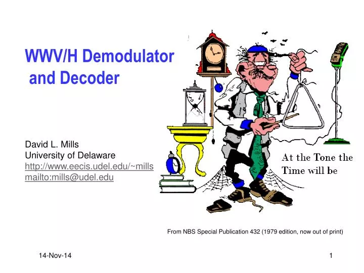
WWV/H Demodulator and Decoder. David L. Mills University of Delaware http://www.eecis.udel.edu/~mills mailto:mills@udel.edu. Class project: a WWV/H receiver demodulator/decoder. Read the paper and read through these slides to see how the various algorithms work.

E N D
WWV/H Demodulator and Decoder David L. Mills University of Delaware http://www.eecis.udel.edu/~mills mailto:mills@udel.edu
Class project: a WWV/H receiver demodulator/decoder • Read the paper and read through these slides to see how the various algorithms work. • Where you can, derive the mathematics involved and work out the various processing gain and probabilities. • Implement as many components as you can in Matlab and verify your calculations match the Matlab simulation. • Hand in your report, including the the Matlab program on the last day of class. • Find a shortwave receiver and dial up one of the transmissions on 2.5, 5, 10, 15 and 20 MHz. See if the sound matches what you would expect from the program.
Program architecture • This program is a mathematically optimum demodulator and decoder for the WWV and WWVH shortwave broadcasts from Colorado and Hawaii. • It operates from the speaker or headphone output of a shortwave radio. • It produces an ASCII timecode suitable for display or as input to another program. • It has been implemented in assembler for the TI 320C25 DSP chip, which includes onboard ADC and DAC chips. • It has been implemented in C as a reference clock driver for the NTP daemon for Unix and suitable sound card or onboard codec. • When used with a tunable radio, it tries all frequencies on a rotating basis and selects the strongest signal.
Transmission format • The transmitted signals are amplitude modulated, double sideband with full carrier. • The transmission format includes 60 slots, each corresponding to one second of the minute. • The first slot contains a 800-ms minute-synch pulse at 1000 Hz for WWV and 1200 Hz for WWVH. It is transmitted at 100 percent modulation. • The remaining slots begin with a 5-ms second-synch pulse at the same frequencies and modulation percentage. • Each slot except the first contains a data pulse at 100 Hz and transmitted at 10 dB below 100 percent modulation. • The minute is divided into six frames of ten seconds. A position marker ends each frame, but these are not used by the program. • Data pulses begin 30 ms into the slot and are width-modulated. • The binary zero pulse is 170 ms wide, binary one 470 ms and position marker (not used) 770 ms. • See the following page for broadcast timecode data decoding.
Voice information • The following two pages, the first for WWV and the second for WWVH describe the voice information included in the transmissions. This includes weather information, status of other navigation services and radio propagation data, including solar flux and magnetic storm indices. • Ordinarily, the voice transmissions do not adversely affect the synchronization recover or data demodulation and decoding functions. The passband filters used by the program further isolate and remove voice frequencies from the spectrum. • For the purpose of performance computations you can ignore the voice modulation and assume the receiver has correctly found minute and second synchronization. Assume synchronous demodulation of the 100-Hz signal and noncoherent demodulation of the 1000/1200-Hz signals.
Synch and data signal demodulation • The following system diagram and spectra show the receiver characteristics. You should calculate the processing gain for all of the components shown. • The IF bandwidth of the communications is 50-2700 Hz. The synch signals are extracted using a narrowband filter, matched filter and comb filter for the second pulse and integrator for the minute pulse. • The data signals are extracted using a lowpass filter and matched filter for the 170-ms data pulse. • Data recovery from the width-modulated pulse uses a slicer, which delivers a pair of probability values, P0 for a zero bit and P1 for a one bit.
Synch and data filtering and demodulation Data Channel 4th-order IIR 170 ms Pulse Width Lowpass Filter0-150 Hz Matched Filter100 Hz ATC and Slicer P0 P1 Receiver IF Bandpass Filter50-2700 Hz 800 ms AF Input Integrator 1000/1200 Hz Minute Pulse Synch Channel 4th-order IIR Bandpass Filter800-1400 Hz 5 ms 1 s Matched Filter1000/1200 Hz Comb Filtert = 1024 s Second Pulse
Second comb filter • The second pulse is shaped by the matched filter and processed by the second comb filter. • Each of 8000 samples is processed once per second by a lowpass filter with time constant ts. • In order to capture the intrinsic oscillator error, ts starts out at 8 and increases eventually to 1024 s. Assume 1024 s in your analysis. To Peak Detector 1/ts Delay 1 s From Matched Filter S 1 – 1/ts
Converting pulse width to probability 200 500 700 P0 P1 P2 285 585 slice level 785 0 870 30 P0 = 0 P0 = 1P1 = 0 P0 = 0P1 = 1P2 = 0 P1 = 0P2 = 1 P2 = 0 • Red shows the matched filter outputs for P0, P1 and P2 (not used). • Blue shows the probabilities assigned to the slice values at negative slice level crossings, where the slice level is set at half the maximum.
Minute comb filter vector Minute Comb Filter Vector • The program cycles through the components of the seconds vector in turn 0-59 s (second 60 only if a leap second is inserted). • Each component is a comb filter for that second of the minute. • Only the fixed data (not clock digits) are updated in this way. • In the current design td is fixed at 16. Second 0 Second 1 … Second 59 Second 60(Leap Sec Only) Output 1/td Delay 1 m From Data Filter S 1 – 1/td
Clock state machine Year Days Hours Minutes • Think of each column of the figure as a wheel rotating about its axis and with the blue color visible as the current time. • The machine works just like a clock with the minute wheel advancing at each minute and where an overflow (e.g., count from 9 to 0) carries to the next higher digit. • Each minute the digits on each wheel are updated by the decoded time. 9 9 9 9 9 9 9 8 8 8 8 8 8 8 7 7 7 7 7 7 7 6 6 6 6 6 6 6 6 5 5 5 5 5 5 5 5 4 4 4 4 4 4 4 4 3 3 3 3 3 3 3 3 3 2 2 2 2 2 2 2 2 2 1 1 1 1 1 1 1 1 1 0 0 0 0 0 0 0 0 0 units tens unts hundreds tensC tens units tens units
Digit correlator 1001 9 • As each data digit is received, the 4 bits are correlated with the corresponding 4 bits of each entry in the coefficient vector and the result exponentially averaged with the corresponding entry in the likelihood vector. • The digit with the maximum probability becomes the maximum likelihood digit for that postion in the timecode vector. • A set of consistency checks suppresses errors. 1000 8 0111 7 0110 6 0101 X = 0101 5 Data 0100 4 0011 3 0010 2 0001 1 0000 0 CoefficientVector LikelihoodVector
Linear filters • The bandpass and lowpass filters on the next two pages were generated in Matlab with the functions and parameters shown. The sample rate is 8 kHz/s. You need to figure out how to use these filters to calculate the processing gain.
Synch channel bandpass filter • 4th-order elliptic 800-1400 Hz bandpass, 8000 Hz sample rate • 0.2 dB passband ripple, -50 dB stopband ripple • Matlab: ellip(4, .2, 50, [800 1400] / 4000)
Data channel lowpass filter • 4th-order elliptic 0-150 Hz bandpass, 8000 Hz sample rate • 0.2 dB passband ripple, -50 dB stopband ripple • Matlab: ellip(4, .2, 50, 150)
Seconds pulses for WWV and WWVH • The leading edge of these pulses marks the beginning of the second. • The modulation percentage is 100 percent. • The other modulating waves are suppressed for the first 30 ms. WWV (1000 Hz) WWVH (1200 Hz)
Seconds pulse autocorrelation function (1000 Hz) • Signal is 5 cycles of 1000 Hz sinewave sampled at 8000 Hz. • What is the level of noise that results in 10 percent error (choosing other than the center peak as the reference second marker?
Seconds pulse crosscorrelation function (1000-1200 Hz) • Signals are 5 cycles of 1000 Hz sinewave and 6 cycles of 1200 Hz sinewave sampled at 8000 Hz. • If the WWV and WVH signals are received, what is the difference (dB) that results in 10 percent error in choosing the wrong station?
Actual performance data • The following diagrams show the performance of the receiver in normal operation, including oscillator frequency, time offset and various performance measures. • Note the daily variation in performance. This is because the frequency in use does not support propagation throughout the day and night. Radio signal propagation conditions were either very good or very bad. Nothing marginal here, except during transition. • The real problem in receiver design is knowing when to abandon the signal and coast through the dark period. Otherwise, the receiver will eat whatever it can, including completely random noise, and result in a high error rate. • Note in the time offset graph that there was in fact some error as the signals came up from noise and the second pulse came out the comb filter up to 12 ms in error. This was fixed by gating off the receiver for 1024 s when coming up from noise.
Oscillator frequency • Note the periods when the oscillator frequency is a horizontal line. This happens when the signal is lost and the oscillator is coasting at its last determined frequency.
Time offset • Note the spikes when the time offset is computed as the signal comes up. This can happen if the oscillator has drifted since last set or because the comb filter has not stabilized.
100 Hz subcarrier SNR • Campare this with the next page. Note that the subcarrier SNR varies a great deal during the day, but the pulse width demodulation acts like an FM receiver, which is relatively insenstitive to amplitude variations.
Digit maximum likelihood amplitude • This is the maximum likelihood digit amplitude. Note the fades during the day when errors might be recognized by the comparison test, which resets the integrator if the digits do not all compare correctly.
Second synch pulse amplitude • This is the master time reference for the driver. It is also the most sensitive to oscillator wander and severe signal multipath.
Minute synch pulse amplitude • Due to the stupendous processing gain, this is usually the first signal to appear and the last to sink beneath the waves.
Further information • NTP home page http://www.ntp.org • Current NTP Version 3 and 4 software and documentation • FAQ and links to other sources and interesting places • David L. Mills home page http://www.eecis.udel.edu/~mills • Papers, reports and memoranda in PostScript and PDF formats • Briefings in HTML, PostScript, PowerPoint and PDF formats • Collaboration resources hardware, software and documentation • Songs, photo galleries and after-dinner speech scripts • Udel FTP server: ftp://ftp.udel.edu/pub/ntp • Current NTP Version software, documentation and support • Collaboration resources and junkbox • Related projects http://www.eecis.udel.edu/~mills/status.htm • Current research project descriptions and briefings