Download
1 / 29
290 likes | 382 Vues
Graphical Display 2. Pictures of Data. Line Graphs. At least two variables, x is often time or depth while the other(s) are plotted for comparison Cumulative graphs allow comparison of two or more distributions ( Quantile comparison plot). > Nelson

E N D
Graphical Display 2 Pictures of Data
Line Graphs • At least two variables, x is often time or depth while the other(s) are plotted for comparison • Cumulative graphs allow comparison of two or more distributions (Quantile comparison plot)
> Nelson Depth Corrugated Biscuit Type_IType_II_RedType_II_YellowType_II_GrayType_III 1 1 57 10 2 24 23 34 5 2 2 116 17 2 64 90 76 6 3 3 27 2 10 68 18 48 3 4 4 28 4 6 52 20 21 0 5 5 60 15 2 128 55 85 0 6 6 75 21 8 192 53 52 1 7 7 53 10 40 91 20 15 0 8 8 56 2 118 45 1 5 0 9 9 93 1 107 3 0 0 0 10 10 84 1 69 0 0 0 0 > NelsonPct <- data.frame(Nelson[,1:2], prop.table(as.matrix(Nelson[,3:8]),1)*100) > NelsonPct Depth Corrugated Biscuit Type_IType_II_RedType_II_YellowType_II_GrayType_III 1 1 57 10.2040816 2.0408163 24.489796 23.4693878 34.693878 5.1020408 2 2 116 6.6666667 0.7843137 25.098039 35.2941176 29.803922 2.3529412 3 3 27 1.3422819 6.7114094 45.637584 12.0805369 32.214765 2.0134228 4 4 28 3.8834951 5.8252427 50.485437 19.4174757 20.388350 0.0000000 5 5 60 5.2631579 0.7017544 44.912281 19.2982456 29.824561 0.0000000 6 6 75 6.4220183 2.4464832 58.715596 16.2079511 15.902141 0.3058104 7 7 53 5.6818182 22.7272727 51.704545 11.3636364 8.522727 0.0000000 8 8 56 1.1695906 69.0058480 26.315789 0.5847953 2.923977 0.0000000 9 9 93 0.9009009 96.3963964 2.702703 0.0000000 0.000000 0.0000000 10 10 84 1.4285714 98.5714286 0.000000 0.0000000 0.000000 0.0000000
# Vital Stats - Crude Birth Rate, Crude Death Rate, Expectancy of # Life at Birth", Infant Mortality, and Total Fertility # Rate from 2000 to 2010 top5 <- c("China", "India", "United States", "Indonesia", "Brazil") Top5<-VitalStats[VitalStats$Country %in% top5, c(substr(colnames(VitalStats), 1, 3) %in% c("IMR", "Cou"))] rownames(Top5) <- Top5$Country Top5$Country <- NULL Top5IMR <- t(Top5) Year <- as.numeric(substr(rownames(Top5IMR), 4, 7)) Top5IMR <- data.frame(Year, Top5IMR) rownames(Top5IMR) <- 1:9 Top5IMR Year United.States Brazil China India Indonesia 1 2000 7.0 35.2 30.3 54.9 40.9 2 2001 7.0 34.0 28.9 51.5 39.5 3 2002 6.9 32.9 27.7 48.2 38.2 4 2003 6.8 31.7 26.4 45.2 36.9 5 2004 6.6 30.7 25.3 42.4 36.4 6 2005 6.5 29.6 24.2 39.7 34.5 7 2006 6.4 28.6 23.1 37.1 33.3 8 2007 6.4 27.6 22.1 34.6 32.1 9 2010 6.2 24.9 19.4 28.1 28.9
Scatterplot – XY Plot • Two interval/ratio variables • Smoothed and regression lines, linear and non-linear relationships • Compare groups (ellipses) • Label points (outliers) • Scatterplot matrix to compare more than two variables
Scatterplot • Numerous options. Turn off all options on the menus, but select “Plot by groups” and select Name • Insert three options into the command: • legend.coords=“topleft” • ellipse=TRUE • levels=.95
ScatterplotMatix • This gives you a visual display of a correlation matrix between three or more variables • Default puts a kernel density plot in the diagonal with a rug showing the data points • For values: by(DartPoints[,6:8], DartPoints$Name, rcorr.adjust)
> library(Rcmdr) > by(DartPoints[,6:8], DartPoints$Name, rcorr.adjust) DartPoints$Name: Darl Length Width Thick Length 1.00 0.59 0.64 Width 0.59 1.00 0.49 Thick 0.64 0.49 1.00 n= 27 P Length Width Thick Length 0.0013 0.0003 Width 0.0013 0.0095 Thick 0.0003 0.0095 Adjusted p-values (Holm's method) Length Width Thick Length 0.0026 0.0009 Width 0.0026 0.0095 Thick 0.0009 0.0095
------------------------------------------------------------ DartPoints$Name: Pedernales Length Width Thick Length 1.00 0.40 0.52 Width 0.40 1.00 0.15 Thick 0.52 0.15 1.00 n= 28 P Length Width Thick Length 0.0365 0.0042 Width 0.0365 0.4611 Thick 0.0042 0.4611 Adjusted p-values (Holm's method) Length Width Thick Length 0.0731 0.0126 Width 0.0731 0.4611 Thick 0.0126 0.4611
3D Scatterplots • Three interval/ratio variables and a possible grouping variable • Often difficult to interpret • Experiment with rotation and view angle • Consider dropping pins to the floor • scatter3d (car) • scatterplot3d (scatterplot3d)
with(DartPoints, scatterplot3d(Length, Width, Thick, type="h"))
Bubble Plot • Bubble plots are scatterplots in which the size of the symbol reflects a third dimension • with(DartPoints, symbols(Length, Width, circles=Thick, inches=1/6, fg="blue", bg="blue")) • ? symbols for more details on the variety of plots possible
> with(DartPoints, symbols(Length, Width, circles=Thick, inches=1/6, fg="blue", bg="blue")) > symbols(c(26, 26), c(35, 33), circles=c(4, 12), inches=1/6, fg="blue", bg="blue", add=TRUE) > text(c(28, 28), c(35, 33), c("Thickness = 4 mm", "Thickness = 12 mm"), pos=4) Create the plot Add circles of min and max size to upper left Add text labels
Publication Quality • In Windows, you can generally save a graph in several formats or place it in the clipboard • For control over resolution and size, plot to a device • Use ?Devices to get the ones available
E.g. Postscript • postscript(file="graph.ps") • plot(rnorm(25), rnorm(25)) • dev.off()
E.g. tif • tiff(file="graph.tif", width=1500, height=1500, res=300, compression="lzw") • plot(rnorm(25), rnorm(25), las=1) • dev.off()
Cairo • Package Cairo gives you access to additional graphic formats including svg as well as some options that are not available in the standard graphics devices.