Download
1 / 11
190 likes | 486 Vues
Smooth Transition Autoregressive Model. Eni Sumarminingsih. Smooth Transition Autoregressive Model. For some process, it may not seem reasonable to assume that the threshold is sharp Smooth Transition Autoregressive (STAR) Model allow the autoregressive parameters to change slowly.

E N D
Smooth Transition Autoregressive Model EniSumarminingsih Eni Sumarminingsih, SSi, MM
Smooth Transition Autoregressive Model • For some process, it may not seem reasonable to assume that the threshold is sharp • Smooth Transition Autoregressive (STAR) Model allow the autoregressive parameters to change slowly. Eni Sumarminingsih, SSi, MM
Consider the special NLAR model given by • If f() is a smooth continuous function, the autoregressive coefficient (α1 + β1) will change smoothly along with the value of Yt-1 • There are two particularly useful forms of the STAR model : the Logistic STAR and the Exponential STAR Eni Sumarminingsih, SSi, MM
The LSTAR Model generalizes the standard AR model such that the AR coefficient is a logistic function : • where • is called the smoothness parameter • In the limit, as --> 0 or ∞, LSTAR become an AR(p) model since the value of is constant. Eni Sumarminingsih, SSi, MM
For intermediate value of , the degree of autoregressive decay depends on the value of Yt-1 • As Yt-1 -, 0 so that the behavior of Ytis given by • As Yt-1 +, 1 so that the behavior of Ytis given by • Thus the intercept and the AR coefficient smoothly change between these two extremes as the value of Yt-1 changes. EniSumarminingsih, SSi, MM
The ESTAR model uses , > 0 • As approach zero or infinity, the model becomes an AR(p) model since is constant • Otherwise, the model display nonlinear behavior • As Yt-1 approach c, approach 0 behavior of Yt is given by Eni Sumarminingsih, SSi, MM
As Yt-1 moves further from c, approach 1 behavior of Yt is given by Eni Sumarminingsih, SSi, MM
Test for STAR Model Step 1 : Estimate the linear portion of the AR(p) model to determine the order and to obtain the residual {et} Step 2 : Estimate the auxiliary equation Eni Sumarminingsih, SSi, MM
Test the significance of the entire regression by comparing TR2 to the critical value of 2. If the calculated value of TR2 exceed the critical value from a 2 table, reject the null hypothesis of linearity and accept the alternative hypothesis of a smooth transition model. Alternatively, you can perform an F test Eni Sumarminingsih, SSi, MM
Step 3 : If you accept the alternative hypothesis (i.e., if the model is nonlinear), test tre restriction a31 = a32 = … = a3p = 0 using an F test. If you reject the a31 = a32 = … = a3p = 0, the model has LSTAR form. If you accept the restriction, conclude that the model has the ESTAR form Eni Sumarminingsih, SSi, MM
Uji F JKGR: JK galat restricted model JKGU: JK galat unrestricted model kU: jumlahpeubaheksogen (termasukkonstanta) pada unrestricted model kR: jumlahpeubaheksogen (termasukkonstanta) pada restricted model Hipotesisnol: restricted model valid Mendugarestricted model danunrestricted model Memperoleh JK Galatuntukrestricted modeldan JK Galatuntuk unrestricted model, danmenghitungstatistikuji F.