Download
1 / 47
470 likes | 572 Vues
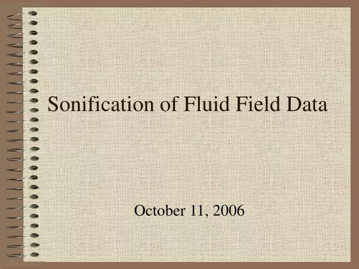
Sonification of Fluid Field Data. October 11, 2006. Outline. Sonification Background Example sonifications General Data specific Project Background Sound options and considerations Specifics Example Further work. Sonification Background.

E N D
Sonification of Fluid Field Data October 11, 2006
Outline • Sonification Background • Example sonifications • General • Data specific • Project • Background • Sound options and considerations • Specifics • Example • Further work
Sonification Background • Sonification is the use of non-speech audio to convey information [B.N. Walker] • Data -> to sound • As an alternative or to complement visual and possibly other displays (e.g.haptic) • Increasing information bandwidth, reinforcement • Recognition of features not obvious from visual displays • Possibility to concentrate on different complementary information by two senses: • Global events through sound, local details through visual cues
Sonification Background • What is being sonified: • General sonification toolboxes • Specific to data sets • Time dependent or static data • How: • Prerecorded sound • Modifying physical properties of sound, pressure, density, particle velocity • Modifying pitch, envelope, duration, timber, etc… • Sonification in real-time or not
Sonification Sandbox [B.N. Walker] • Input: several data sets in a form of MxN matrix • Each data set can be mapped to pitch, timbre, volume, or pan. One dataset mapped to time. • GUI for user manipulation of mappings • Length that each data point is played corresponds to the relative spacing of the data points in the time dimension • Program download: http://sonify.psych.gatech.edu/research/sonification_sandbox/sandbox.html Sonification Example I
Data Sonification and Sound Visualization [H.G. Kaper] • Sonification • DIASS (a Digital Instrument for Additive Sound Synthesis) • Sound by summation of simple sine waves: • Static and dynamic control parameters applied at the level of partials and collected sound • Various mappings from the degrees of freedom in the data to the parameters Sonification Example II
Data Sonification and Sound Visualization • Sonification (cont’d) • Creating sound not real time • Sound examples: http://www-unix.mcs.anl.gov/~kaper/Sonification/DIASS/Demos/index.html • Sound visualization • To detect sound structure • One-to-one mapping between control parameters and visual attributes • Done in real time Sonification Example II
Visualization (cont’d) The grid indicates the frequency spectrum 8 octaves, corresponding approximately to the range of a piano Partials mapped to spheres: Diameter - amplitude Height - frequency Colors - amount of reverberation Data Sonification and Sound Visualization Sonification Example II
Sonification of time dependent data[M. Noirhomme-Fraiture] • 2D and 3D time-dependent graphs • Value to frequency • Discard outliers • Pre-smooth curves • Their experiments show that having a musical or a computer science background gives a minor advantage in using sonification of 2D curves and no difference for the 3D case Sonification Example III
Cell Music [K. Metze]: • Sonification of Digitalized Fast-Fourier Transformed Microscopic Cell Images: • Luminance of each pixel to amplitude • Distance from the central point to spatial frequency • Vector is moving clockwise from 0 to 6 hour position. Sound of each pixel is played when the vector strikes it • Sound duration is inversely proportional to frequency • Most important frequencies filtered out • Geodesic reconstruction: method defining subregions in FFT image around regional maxima with a luminance difference up to 3 gray levels lower Sonification Example IV
Cell Music Lower frequencies predominate in malignant cells, thus these cells can be easily recognized in the cell sound as slowly moving chords of lower frequencies with intense amplitudes Sonification Example IV
Heart Rate Sonification [M. Ballora] • Interbeat interval characteristics are mapped to sound characteristics • Sound files and sonification mapping overview: http://www.music.psu.edu/Faculty%20Pages/Ballora/sonification/sonex.html Electrocardiographic recording of the heartbeat. Sonification Example V
LHEM for Interactive Sonification[T. Bovermann]: • Local Heat Exploration Model: • Data Selection: • An item x is selected if it is inside the selection aura • Exploration Model: dynamical model whose configuration is determined by selected data • Data items has position, feature and heat • Feature vectors similar to each other produce high heat values, dissimilar – lower ones Sonification Example VI
LHEM for Interactive Sonification: • Exploration Display: • Superimposing lots of short grains (~5ms) to compose a grain cloud • grain cloud parameters: • Example explorations: • Example sound files: http://www.techfak.uni-bielefeld.de/~thermann/projects/ Sonification Example VI
Vortex Sound Synthesis [Y. Shin] • 3D time-varying scalar field data. Sound propagating from sound sources • Physically-based sound synthesis: data is mapped to acoustic parameters like density and particle velocity Sonification Example VII
Vortex Sound Synthesis • Three steps: • Synthesis: capture user movement, compute sounds generated by the sources • Rendering: compute sound heard by the listener, taking into account effect like sound source distance • Localization:virtual sounds mapped to a distribution of audio signals for real world speakers • Example movie file: • http://www.cs.utexas.edu/~bajaj/explosion(sound).mpg Sonification Example VII
Sonification of Numerical Fluid Flow Simulations [E. Childs] • Real-time sonification of CFD solution process • To gain insight into the solver by listening to its progress • Mappings • Pitch Mapping: velocity values in x and y dimension are mapped to frequency and major triads • Envelope: attack, sustain and decay derived from the matrix coefficients for each variable at each node • Delays between nodes, columns, at the end of each iteration to convey calculation stage Sonification Example VIII
Sonification of Numerical Fluid Flow Simulation, example • Two-dimensional developing flow in a planar duct • 5 x 5 = 25 internal or “live” cells at which the values of u, v and p are updated at each iteration by the solver • The solver converges in about 20 iterations • Sound file: • http://eamusic.dartmouth.edu/~ed/sounds/CFDSound2.mp3 Sonification Example VIII
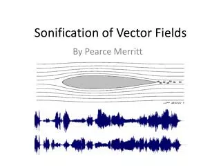
Sonification of Vector Fields [E. Klein] • Rectilinear grids of vectors • A sphere at the listener’s position. Random samples within that sphere • Mapping vector direction and magnitude of sampled particle: • Vector direction to sound location • Vector magnitude to sound level and pitch Sonification Example IX
Sonification of 3D Vector Fields Two consecutive vector samples taken at random locations within the listener’s head volume Hermite curve to achieve C1 continuity between two sound positions Sonification Example IX
Sonification of 3D Vector Fields • Vorticity (turbulence) in the sampled area: • All of the samples in the area are roughly the same magnitude and direction: constant and smooth sound – low vorticity • Vectors vary widely: sound appears to shift more, giving the impression of higher turbulence • Size of the sample volume in relation to the density of the vectors within the field plays an important role Sonification Example IX
Project Background • Input: • Fluid field with velocity vector, pressure, plus potentially density, temperature and other data • Changes with time • Output: • Sound characterizing the given fluid field • Ambient: global to the whole field • Local: at the point or area of interaction
Project: sound options • Global • Every particle in the field contributes to the sound • The further sound source is from the virtual pointer the less contribution it makes, the quieter it is • Local point • Only the field characteristics at the virtual pointer position contribute to the sound • Local region • Particles of the specific subset area around the pointer contribute to the sound • Possibility to add zoom factor to expand or contract the space of interaction
Project: sound options • Sonification along the pathlines, streaklines, streamlines, streamtubes • Map field characteristics along above traces to the sound parameters • Possibly starting from the point of virtual pointer • Map changes in the streamtube appearance to the changes in sound parameters (twist, direction, cross-sectional area radius etc…) • In an unsteady flow, streamlines, streaklines, and pathlines are not necessarily the same. In a steady flow, however, all three lines coincide [C.Wassgren]
Definitions [by C.Wassgren] • Pathline: • A line that a single particle traces out over time. A line you get from a long exposure photograph highlighting a single particle • Streakline: • The locus of all particles that have passed through a prescribed fixed point during a specific interval of time. A line traced by the continuous injection at a certain point of dye, smoke, or bubbles • Streamline: • A curve everywhere tangential to the instantaneous velocity vectors, that is, everywhere parallel to the instantaneous flow direction • Demonstration: http://widget.ecn.purdue.edu/~meapplet/java/flowvis/Index.html
Sound parameters • Possibility to map field data to: • Frequency, Pitch • Duration, Envelope – attack, sustain and decay of sound • Spatial location – direction of were the sound is coming from • Loudness, intensity, amplitude of vibration • Timbre, consonance, dissonance, beats, roughness, density, volume, vibrato, silence pauses
Psychoacoustics • Sound parameters require a certain percentage of change for the change to be noticed, examples: • Minimum audible angle • Minimal intensity change • Tone duration • Softer tone is usually masked by a louder tone if their frequencies are similar • Relation between subjective sound traits and their physical representations • Loudness relation to intensity and frequency
Psychoacoustics • Curves of equal loudness level:
Project specs • Components (hardware, software, libraries): • Max/MSP: mapping data values to sound • Omni Haptic Device: navigation through 3D fluid data • SGI OpenGL Performer Library: graphical representation of the given field and virtual pointer • Quanta libraries: to read data from the main server • VRPN libraries: connections between different parts of the program
Solution Data Server Visualization Program Main Program as Max/MSP object Haptic Program Image Sound Haptic Device Structure • Each rendering program is independent of any other Max/MSP Program
Haptic Program • Read from the haptic device • Position • Orientation • Buttons • Converts the position to the data field coordinates • Sends pointer info to the sound and visual programs • Pointer position • Pointer orientation • Interaction sphere diameter - local region
Haptic Program • Gives a force feedback: • Creates virtual walls of the dataset • Provide a force disallowing movement of the device outside of the data field boundary • Other feedback possible • Produce a force that is proportional to the flow density and its direction
Visualization program • Receives dataset from the Solution Data Server • Receives virtual pointer position & orientation, as well as sphere diameter from the haptic program • Displays vector field, virtual pointer (microphone) and interaction sphere:
Max/MSP • Max/MSP is a graphical programming environment for sound manipulation • Allows you to write your own objects • Large capability for a very sophisticated program • Various built in audio signal processing objects: • noise~ - generates white noise • reson~ - filters input signal, given center frequency and bandwidth • *~ - product of two inputs, in given case scales a signal’s amplitude by a value
Max/MSP object • Receives dataset from the Solution Data Server • Receives virtual pointer position & orientation, as well as sphere diameter value from the haptic program • Calculates velocity vector at the position of the virtual microphone Depending on interaction sphere radius: • Small : from vertices of the grid cell • Large: from all the vertices inside the influence sphere
Max/MSP object • Calculates velocity vector at the position of the virtual microphone using Schaeffer’s interpolation scheme: • From velocity vector at the point of interaction: • velocity value at the position of the virtual cursor • angle between pointer vector and velocity vector
Max/MSP object • Two output values for both angle and velocity: • Output = value / max value • Output = (value / max value) 5/3 • Relationship between loudness level and intensity: S ~ a3/5 [B.Gold] Thus, a function between values and amplitude should be: a = const * data value5/3 to imply S ~ data value
Max/MSP program white band noise is modified in amplitude and frequency to simulate a wind effect: Frequency ~ , were v -> [0,1] -> [500, 1500] Amplitude ~ * 5/3, were v5/3-> [0,1] and a5/3-> [0.5, 1]
Further work • Refining the program • Mesh in the visual program • Possible other set-ups for Max/MSP sound program • Using headphones or speakers to convey spatial sound • Experiments
Sound Localization • HRTF ( Head-Related Transfer Functions) • Describes changes in amplitudes and phases of a sound as it travels from a sound source towards the outer ear [W.A. Yost] • ILD – interaural level difference • IPD – interaural phase difference • ITD – interaural time difference • Intracranial (occurring inside the listener’s head) lateralization (right to left) vs. extracranial (occurring in space) localization (azimuth, vertical and distance spatial dimensions)
Horizontal HRTF [12] Spectrum of sound depends on the direction it came from [S.A. Gelfand]
Further work • Refining the program • Experiments • Goals of experiments • Defining experiments • Setting up experiments • Collecting useful information • Sound has to convey useful information to the listener
References [1] B.N. Walker, J.T. Cothran, July 2003, Sonification Sandbox: a Graphical Toolkit For Auditory Graphs, Proceedings of the 2003 International Conference on Auditory Display, Boston, MA [2] H.G. Kaper, S. Tipei, E. Wiebel, 5July 2000, Data Sonification and Sound Visualization [3] K. Metze, R.L. Adam, N.J. Leite, Cell Music: The Sonification of Digitalized Fast-Fourier Transformed Microscopic Images [4] M. Ballora, B. Pennycook, P.C. Ivanov, L.Glass, A.L. Goldberger, 2004, Heart Rate Sonification: A New Approach to Medical Diagnosis, LEONARDO, Vol. 37, No. 1, pp. 41–46 [5] M. Noirhomme-Fraiture, O. Schöller, C. Demoulin, S. Simoff, Sonification of time dependent data
References [6] Y. Shin, C. Bajaj, 2004, Auralization I: Vortex Sound Synthesis, Joint EUROGRAPHICS - IEEE TCVG Symposium on Visualization [7] E. Childs, 2001, The Sonification of Numerical Fluid Flow Simulations, Proceedings of the 2001 International Conference on Auditory Display, Espoo, Finland, July 29-August 1 [8] E. Klein, O.G. Staadt, 2004, Sonification of Three-Dimensional Vector Fields, Proceedings of the SCS High Performance Computing Symposium, pp 8 [9] G. Kramer, B. Walker, T. Bonebright, P. Cook, J. Flowers, N. Miner, J. Neuhoff, R. Bargar, S. Barrass, J. Berger, G. Evreinov, W.T. Fitch, M. Gröhn, S. Handel, H. Kaper, H. Levkowitz, S. Lodha, B. Shinn-Cunningham, M. Simoni, S. Tipei, Sonification Report: Status of the Field and Research Agenda, http://www.icad.org/websiteV2.0/References/nsf.html
References [10] C.Wassgren, C.M. Krousgrill, P. Carmody, Development of Java applets for interactive demonstration of fundamental concepts in mechanical engineering courses,http://widget.ecn.purdue.edu/~meapplet/java/flowvis/Index.html [11] W.A. Yost, 2000, Fundamentals of Hearing: An Introduction, Forth Edition [12] S.A. Gelfand, 2004, Hearing: An Introduction to Psychological and Physiological Acoustics, Forth Edition, Revised and Expanded [13] T. Bovermann, T. Hermann, H. Ritter, July 2005, The Local Heat Exploration Model for Interactive Sonification, International Conference on Auditory Display, Limerick, Ireland [14] B. Gold, N. Morgan, 2000, Speech and Audio Signal Processing: Processing and Perception of Speech and Music