Download
1 / 21
210 likes | 212 Vues
Learn how differential equations can be used to model population growth and other changing quantities. Solve systems of differential equations and explore different scenarios.

E N D
Recall from AP Calculus The number of rabbits in a population increases at a rate that is proportional to the number of rabbits present (at least for awhile.) So does any population of living creatures. Other things that increase or decrease at a rate proportional to the amount present include radioactive material and money in an interest-bearing account. If the rate of change is proportional to the amount present, the change can be modeled by:
Rate of change is proportional to the amount present. Divide both sides by y. Integrate both sides.
Integrate both sides. Exponentiate both sides. When multiplying like bases, add exponents. So added exponents can be written as multiplication.
Since is a constant, let . Exponentiate both sides. When multiplying like bases, add exponents. So added exponents can be written as multiplication.
At , . Since is a constant, let . This is the solution to our original initial value problem.
So if we start with: We end with:
What if we have a series of differential equations? We could solve these individually y1 =c1ekt y2 =c2ekt y3 =c3ekt Provided that we have initial conditions for each of these to solve for the constants.
If we define x [ ] x1’(t) x’(t) = x2’(t) xn ’(t) This yields the equation x’(t)= Ax Which is easy to solve in the case of a diagonal matrix. … [ ] [ ] [ ] x1 x2 x3 x’1 x’2 x’3 • 0 0 • 0 -2 0 • 0 0 4 = We can solve each of these as a separate differential equation x1’ = 3x1, x2’ = -2x2, x3’ = 4x3 x1 (t) = b1e3t, x2 (t) = b2e-2t, x3 (t) = b3e4t, This is the general solution. We can solve for the constants if given an initial condition.
First order homogeneous linear system of differential equations x1’(t) = a11x1 (t) + a12 x2 (t) + … a1nxn (t) x2’(t) = a21x1 (t) + a22 x2 (t) + … a2nxn (t) xn ’(t) = an1x1 (t) + an2 x2 (t) + … annxn (t) … [ ] [ ] We could write this in matrix form as: x1’ (t) a11 a12 …. a12 x(t) = x2’ (t) A = a21 a 22 … a2n xn’ (t) an1 a n2 …anm … …
What if our system is not diagonal? du1 = -u1 + 2u2 dt du2 = u1 – 2u2 dt The system at the left can be written as du/dt = Au with a as [ ] A = -1 2 1 -2 [ ] How can we solve this system? 1 0 Initial condition u(0) =
du/dt = Au y = eAt u(t) = c1eλ tx1 +c2e λ tx2+…+ cneλ txn Check that each piece solves the given system du/dt = Au d (eλ tx1) = A eλ tx1 λeλ tx1 = A eλ tx1 dt λx1 = Ax1 n 2 1
Key Formulas Difference Equations Differential Equations du/dt = Au y = eAt
Solve the differential equations The system at the left can be written as du/dt = Au with a as Start by computing the eigenvalues and eigenvectors [ ] A = -1 2 1 -2 What are the eigenvalues from inspection? Hint: A is singular The trace is -3
Solve the differential equationsStep 1 find the eigenvalues and eigenvectors We can a solve via finding the determinant of A - λI By inspection: the matrix is singular therefore 0 is an eigenvalue the trace is -3 therefore the other eigenvalue is -3. [ ] det -1-λ 2 1 -2-λ Calculate the eigenvector associated with λ = 0, -3 [ ] [ ] 2 1 A = -1 2 1 -2 For λ = 0 find a basis for the kernel of A For λ= -3 find a basis for the kernel of A+3I [ ] [ ] 1 -1 A+ 3I = 2 2 1 1
Solve the differential equations The system at the left can be written as du/dt = Au with a as Note: the solutions of the equations are going to be e raised to a power. [ ] A = -1 2 1 -2 The form that we are expecting for the answer is y = c1 e λ t x1 + c2 e λt x2 1 2 The eigenvalues are already telling us about the form of the solutions. A negative eigenvalue will mean that that portion goes to zero as x goes to infinity. An eigenvalue of zero will mean that we will have an e0 which will be a constant. We will call this type of system a steady state.
Solve the differential equations Solve by plugging in eigenvalues into expected equation and for λ1 and λ2. and the corresponding eigenvectors in x1 and x2 y = c1 e0t 2 + c2 e -3t 1 1 -1 [ ] A = -1 2 1 -2 [ ] [ ] We find c1 and c2 by using the initial condition Plugging in zero for t and the initial conditions yields: [] Recall: 1 0 [] [ ] [ ] Initial condition u(0) = 1 = c1 2 + c2 1 0 1 -1 c1 = 1/3 c2 = 1/3
Solve the differential equations The general solution is y = 1/3 2 + 1/3 e -3t 1 1 -1 [ ] [ ] We are interested in hat happens as time goes to infinity Recall our initial condition was 1 all of our quantity was in u1 0 Then as time progressed there was flow from u1 to u2. As time approaches infinity we end with the steady state 2/3 1/3 [] [ ]
The solution to y’ = ky is y = y0ekt The solution to x’ = Au is u = c0eAt
What if the matrix is not diagonal? • White book p. 520 ex 3, 4, 5