Download
1 / 36
360 likes | 368 Vues
This segment covers the basics of sampling and inference, including ways to describe and characterize data, the importance of random sampling, moments of the sample mean, and making inferences about a population from a given sample. The Central Limit Theorem and examples of probability calculations are also discussed.

E N D
Statistics and Quantitative Analysis U4320 Segment 5: Sampling and inference Prof. Sharyn O’Halloran
Sampling • A. Basics • 1. Ways to Describe Data • Histograms • Frequency Tables, etc. • 2. Ways to Characterize Data • Central Tendency • Mode • Median • Mean • Dispersion • Variance • Standard Deviation
Sampling(cont.) • 3. Probability of Events • If Discrete • Rely on Relative Frequency • If Continuous • Rely on the distribution of events • Example: Standard Normal Distribution • 4. Samples • We can take a sample of the population and make inferences about the population. • 5. Central Question • How well does the sample represent the underlying population?
Sampling (cont.) • B. Random Sampling • 1. Problems with Sample Bias • The way we collect our data may bias our results. That is, the average response in our sample may not represent the average response in the whole population. • Examples: • Literary Digest Phone Book Poll • Primaries • Relation between economic growth and education looking only at OECD countries • 2. Solution • Random Sampling
Sampling (cont.) • C. Moments of the Sample • 1. Characteristics of Sample Mean
Sampling (cont.) • Example • Draw a single observation
Sampling (cont.) • Draw two observations
Sampling (cont.) • Draw 4 Observations
Sampling (cont.) • 2. Generalization • Every sample has an expected mean of . • But as our sample size increases, we are more confident of our results. • That is, the standard deviation (or standard error as we will call it) of our results is decreasing. • So as N increases,
Sampling (cont.) • 3. Hat Experiment • Mean = 10.5 • Standard deviation s = 5.77 • Now let's take a sample of size 1. (With replacement.) • Now one of size 2. • Now one of size 6.
Sampling (cont.) • 4. Equations • For a sample of size n from a population of mean and standard deviation , the sample mean has: • SE( ): it's called the standard error of the sampling process.
Inference We make inferences about a population from a given sample. • A. Population and Sampling Parameters • We have a population with parameters and . • We then take a sample with parameters and s. • We want to know how well the sample mean approximates the population mean .
Inference (cont.) • On average the sample mean equals the population mean.
Inference (cont.) • B. Referring Back to the Hat Experiment • 1. Sample Error decreases as n increases • For instance, before we drew samples of sizes 1, 2, and 6 from the hat. • The first sample of size 1 had standard error 5.77/ 1 = 5.77. • The second sample of size 2 had standard error 5.77/ 2 = 4.08. • The third sample of size 6 had standard error 5.77/ 6 = 2.36.
Inference (cont.) • C. Shape of the Sampling Distribution • If you take a sample and find its mean, then take another sample and find its mean and repeat this process a large number of times then • is a random variable with its own mean and standard error.
Inference (cont.) • 1. Central Limit Theorem • Take a large number of samples, then, the sample mean is normally distributed with mean and standard error .
Inference (cont.) • 2. Example: 3 different distributions • Example 1; • A population of men on a small, Eastern campus has a mean height =69" and a standard deviation =3.22". If a random sample of n=10 men is drawn, what is the chance that the sample mean will be within 2" of the population mean?
Inference (cont.) • Answer: • From the Central Limit Theorem, we know that is normally distributed, with mean 69 and standard error:
Inference (cont.) • Answer (cont.) • Find z-score • P(Z>1.96) = 0.025. Since there are two tails, the area in the middle is: So there's a 95% probability that the sample mean falls between 67 and 71.
Inference (cont.) • Example 2: • Suppose a large class in statistics has marks normally distributed around m = 72 with s = 9. Find the probability that • a) An individual student drawn at random will have a mark over 80.
Inference (cont.) • Answer: • The Z-score is (80-72)/9 = .89 • Looking this up in the table gives P(Z>.89) = .187, or about 19%. • b) Now, what's the probability that a sample of size 10 has an average of over 80?
Inference (cont.) • Answer: • The standard error is = 9/ 10 = 2.85. • So the Z-Score becomes (80-72)/2.85 = 2.81. • P(Z> 2.81) = .002.
Inference (cont.) • Example 3: I • f the number of miles per gallon achieved by all cars of a particular model has m = 25 and s = 2, what is the probability that for a random sample of 20 such cars, average miles per gallon will be less than 24? (assume that the population is normally distributed.) • Step 1: Standardize X
Inference (cont.) • Step 2: Then Find the Z scores (From the standard Normal tables) • So there is about a 1.3 percent chance that from a sample of 20 the average will be less than 24.
Inference (cont.) • D. Proportions • 1. Proportions as Means • A proportion (P) is just the mean of a dichotomous variable. • Example • Ask 50 people what they think of Clinton; • 0 if think he's doing a poor job; and • 1 if think he is doing a good job. • Suppose 30 of the 50 respondents say he's doing a good job • Then, the sample mean P is 30/50 = .60. • This is just another way of saying that 60% of those surveyed approved of his job performance.
Inference (cont.) • 2. Formula for Standard Error • For a large enough sample of size n, P (the proportion) will be normally distributed with mean and standard deviation . • Population Mean = Population Proportion • Sample Mean = Sample Proportion P • Population SD =
Inference (cont.) • 3. Example: Polling • Suppose that the true approval rating for Clinton is .50. That is, 50 percent of the population believe he is doing a good job. = .5 • If we sample 50 people, what is the probability that we will observe an approval rating as high as 60 percent or above?
Inference (cont.) • We know that the true population mean is =.5, • The Standard Error = = 0.0707 • Then the Z-score is (.6-.5) / 0.0707= 1.414 • Looking this up in the Z-table, P(Z>1.414) = .079, or about 8 %.
Inference (cont.) • 4.Example • Of your first 15 grandchildren, what is the chance that there will be more than 10 boys?
Inference (cont.) • Answer: • What the probability is that the proportion of boys is at least 10/15=2/3. • We know that the population mean is =1/2, • The standard error = • Then the Z-score is (.667-.5) / 0.129 = 1.29. • Looking this up in the table, P(Z>1.29) = .099, or about 10%.
Point Estimation: Properties • A. Unbiased Estimators • When an estimator has the property that it converges to the correct value, we say that it is unbiased.
Point Est. Properties (cont.) • B. Efficient Estimators • Def of Efficient: One estimator is more efficient than another if its standard error is lower.
Point Est. Properties (cont.) • C. N-1 Problem • 1. Known • When we take a sample of size n, if we had the real from the population, we could calculate • Then there wouldn't be a problem; would be a consistent estimator of , if we knew .
Point Est. Properties (cont.) • 2. Unknown • But we usually don't have , so we have to use the sample mean instead. What's the difference? Why don't we just say that • It turns out that we can show that minimizes the expression .
Point Est. Properties (cont.) • 2. Unknown (cont.) • So if we used instead, then, the expression would be bigger. • The right way to correct for this is to multiply by , so • The bottom line is that we use n-1 to make a consistent, unbiased estimate of the population variance.
IV. Review Homework • IV. Review Homework