Download
1 / 30
310 likes | 317 Vues
This study presents an analysis of congestion costs in Edmonton, Canada using a transportation demand model. The model considers the implementation of congestion pricing and examines the changes in composite utility to assess the impact on travel demand.

E N D
Estimating Congestion Costs Using a Transportation Demand Model of Edmonton, Canada C.R. Blaschuk Institute for Advanced Policy Research University of Calgary A.T. Brownlee Transportation Department City of Edmonton J.D. Hunt Institute for Advanced Policy Research University of Calgary Presented at the 11th TRB National Transportation Planning Applications Conference Daytona Beach, FL May 8, 2007
Outline • Introduction • Overview of Congestion Pricing • Edmonton Model • Method • Scheme considered • Modifying Volume-Delay Functions • Composite Utility Approach • Results
Introduction Goals • Quantify total economic costs from congestion • Theoretical viewpoint only • Use values as a basis for further consideration • Easy implementation in an existing model • Results from a model used in everyday engineering applications • Useful results
Introduction Quantifying Congestion • Two approaches • Engineering • Differences from free-flow or acceptable conditions • Economic • Deadweight losses due to inefficient pricing of roads • Economic approach used
Demand Marginal Total Costs generalized cost Average Private Costs A J C H K B G F L M D E O flow of vehicles Market view of flow of vehicles on a section of roadway; with congestion deadweight loss shown Economic Approach
Demand Marginal Total Costs generalized cost Average Private Costs A J C H K B G F L M D E O flow of vehicles Market view of flow of vehicles on a section of roadway; with congestion deadweight loss shown Unpriced Equilibrium
Demand Marginal Total Costs generalized cost Average Private Costs A J C H K B G F L M D E O flow of vehicles Market view of flow of vehicles on a section of roadway; with congestion deadweight loss shown Gap in costs (cost to society vs cost driver pays)
Demand Marginal Total Costs generalized cost Average Private Costs A J C H K B G F L M D E O flow of vehicles Market view of flow of vehicles on a section of roadway; with congestion deadweight loss shown Priced Equilibirum Tolls Collected
Demand Marginal Total Costs generalized cost Average Private Costs A J C H K B G F L M D E O flow of vehicles Market view of flow of vehicles on a section of roadway; with congestion deadweight loss shown Deadweight Loss (DWL)
Introduction Used the Regional Transportation Model of Edmonton, Canada Base Conditions
Introduction Edmonton Regional Transportation Model (RTM) • Built in EMME/2 • 1,091 Zones, 15,400 Links • Enhanced 4-Step Model • Rich feedback mechanisms • Time of Day and Peak Spreading • 24 Hours (5 Time Periods) • 25 Person Group / Trip Type Combinations • Ex. Adult Home-to-Work, Adult Work-to-Home, etc • Nested Logit Structure
24 Hour Trip Destination Choice: origin zone i j(1) j(2) .... j(n) destination zone j ò Time of Day Choice: daily i-j am off pm ò Mode Choice: time of day i-j metabolic mechanical auto cycle transit walk car p&r car1 car2 car3 ò Peak Crown vs Peak Shoulder Choice: car mode i-j peak crown peak shoulder Conceptual nested logit model structure
Method • Apply congestion charges network-wide • Toll all auto links to prevent toll evasion • Can calculate theoretical maximum costs • No tolls for public transit • Implement tolls by modifying volume-delay functions • VDFs represent average costs AC(v) at volume v • Total costs TC(v) = AC(v)*v • Marginal costs MC(v) = d[TC(v)]/d[v]
Method Two runs needed • Base – 2005 Model • Congestion Pricing – Apply Marginal Cost Functions to Base 2005 model • First look at results on a link-based level
Method Findings • Volumes typically decreased on major links with addition of tolls. • Volumes sometimes increased on minor links with addition of tolls. • End result: demand is shifting • Link based analysis not an appropriate method • Not possible to calculate system-wide deadweight loss
Marginal Total Costs Base Demand generalized cost Average Variable Costs O D E flow of vehicles
Method Why would demand shift? • Network-wide toll increases desire to make shorter trips (to closer destinations) • Desire to travel at different times of day and use different modes • Increased costs on less congested links less than increases on more congested links.
Method Need to look at costs where demand wont shift • Assume demand for travel stays the same • Look at changes in composite utility • Composite Utility provides information on costs of choices from all alternatives at lower levels in the nested logit model • Composite Utility of accessibility to Origins/Destinations is part of trip generation level in the logit model • Can look at changes in the composite utility of accessibility to determine how much travel is changing without changing demand for travel.
Method Calculating Composite Utility of Accessibility • Need 4 Points • CU for base case • CU for congestion pricing case • What CU would be with congestion pricing at base volumes • What CU would be with base pricing at congestion pricing volumes
Demand Marginal Total Costs generalized cost Average Private Costs A J Want composite utility for these points C H K B G F L M D E O flow of vehicles Market view of flow of vehicles on a section of roadway; with congestion deadweight loss shown
Method • Know composite utility from cases 1 and 2 (part of model run calculations). • For case 3 • Replace average costs with marginal costs • Reassign to get new travel costs • Recalculate composite utility based off new travel costs • For case 4 • Replace marginal costs with average costs • Reassign to get new travel costs • Recalculate composite utility based off new travel costs
Method • Results measured in changes of composite utility values • To convert to dollars • Raise operating costs by $1 • Observe change in utilities corresponding to $1 change to get change in utility/$ • Using change in utility and volumes, can obtain all necessary values.
Results • Decrease in auto trips across the day • Some peak spreading evident • PM experienced biggest losses • Likely most congested time of day • Transit absorbs most of the displaced auto trips • About 5,700 trips leave the system
Results • Total daily tolls collected is ~$750,000 / day • Comparable to other studies • Daily deadweight loss of ~$1,300 / day • Seems low at first glance • Increasing inputs by 30% lead to a deadweight loss of $7,000 / day • An increase of over 500%
Results • Deadweight loss values low, but magnitude comparable to other studies • Limited previous work calculating deadweight loss values • Focus has been more on ‘eliminating’ deadweight loss by calculating tolls collected and costs to drivers.
Results • Possible reasons for a low deadweight loss • Most congestion in Edmonton could be efficient • Edmonton might not be that congested • Large amount of capacity in transportation system that could absorb most of the congestion pricing impacts
Results • Must keep in mind the difference in definition of congestion costs • Engineering costs calculated from composite utility approach to be ~$180,000 / day • Would equal about $45 million / year for weekdays only • Much different from economic costs, but is really answering a different question than the economic approach
Conclusions • Deadweight loss can be used as an initial criteria for consideration of congestion pricing schemes • Value may be too small for Edmonton • Deadweight loss looks to make up a very small part of the costs of congestion using this approach • Suggests most congestion is efficient • Further application of method on models of other cities may reveal more about deadweight loss