Download
1 / 39
420 likes | 678 Vues
Estimating Demand Functions. Chapter 4. 1. Objectives of Demand Estimation. determine the relative influence of demand factors. forecast future demand. make production plans and effective inventory controls. 2. Major approaches to Demand Estimation. a. Marketing Research.

E N D
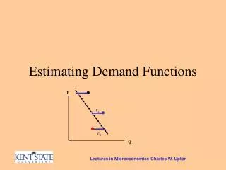
Estimating Demand Functions Chapter 4
1. Objectives of Demand Estimation • determine the relative influence of demand factors • forecast future demand • make production plans and effective inventory controls
2. Major approaches to Demand Estimation a.Marketing Research • Consumer survey) (telephone, questionnaire, interviews, online survey)
Advantage: provides useful data for the introduction of new products Disadvantages: • It could be biased due to unrepresentative sampling size • Consumers may provide socially acceptable response rather than true preferences
Consumer Clinic • a sample of consumers is chosen either randomly, or based on socio-economic features of the market • They are given some money to spend on goods • Their purchases are being observed by a researcher
Advantages: • more realistic than consumer surveys • avoids the shortcomings of market experiments(costs). Disadvantages: • participants know that they are in anartificial situation • small sample because of high cost
Market Experiments • Similar to consumer clinic, but are conducted in an actual market place • Select several markets with similar socio-economic characteristics and change a different factor in each market • Use census data for various markets and study the impacts of differences in demographic characteristics on buying habits
Market Experiments : Advantages • Can be done on a large scale • Consumers are not aware that they are part of an experiment
Problems of Marketing Research • the sample may not be representative • Consumers may not be able to answer questions accurately-biased
2b.Statistical Method • Involves the use of regression analysis to determine the relative quantitative effect of each of the demand determinants. Regression Analysis is usually: • more objective than marketing research • provides more complete information than market research • less expensive
3. Steps in regression analysis • Specify the model (theory) • Obtain data (types and sources) • Specifying the form of the demand equation (linear, log linear) • Specifying the form of the demand equation (linear, log linear) • Estimate the regression coefficients (Finding the line of best fit by minimizing the error sum of squares) • ∑(Yt – )2 = ∑(Yt - a - bXt)2 =0
Steps in Regression Analysis contd • Test the significance of the regression results (Overall tests and individual tests). • Use the results of the regression analysis as a supporting evidence in making business policy decisions (change price, ad strategy, customer service)
4 a.Given Sales (Yt in ‘000 units) and Advertising Expenditures (Xt) (in mill. $) data as follow:
a. b.
4c. Interpretation of Regression Coefficients -- is the intercept term which represents the value of the dependent variable when Xt=0. -- has no economic meaning when its value lies outside the range of observed data for Yt. Note: Data Range=> 25-63
- the slope of the regression line - represents the change in the dependent variable (Yt) related to a unit change in the independent variable =5.14 means that a $ 1 million dollar increase in ad expenses will result in an increase in sales by 5140 units.
4d. Overall Measures of Model Performance • R2=coefficient of determination • = the ratio of the variation in sales explained by the variation in ad expenses. • =Explained Variation/Total Variation
Notice that R2 is adjusted for the degrees of freedom- the number of observations beyond the minimum needed to calculate a given regression statistic. For example, to calculate the intercept term, at least one observation is needed; to calculate an intercept term plus one slope coefficient, at least two observations are required, and so on.
=>Explained variation =>Total variation =.761 means that 76.1% of the variation of in sales is explained by the variation in advertising expenditures.
Note:One would like R2 to be as high as possible. R2, however, depends on the type of data used in the estimation. It is relatively higher for time series and smaller for cross-sectional data. For a cross-section data, R2 of .5 is acceptable.
(ii) F-Statistic F-Statistic- a statistical test of significance of the regression model. F- Test of Hypotheses Decision Rule: Accept Ho if F-calculated < F-table Reject HO if F-calculated> F-table
F-table is defined for df1=k-1, df2=n-k) at a= .05 (conventional) or a=.01, or any other level of significance. [k= # of parameters (2), n= # of observations (7)] F(1, 5) at a= .05 = 6.61, F-cal= R2/k-1/[(1-R2)/(n-k)] =.751/.249/5=15.1 Reject Ho since F-cal>F-table, i.e. the regression model exhibits a statistically significant relationship.
4e. The t-statistic test is a test of the individual independent variable. • T- test of hypotheses
Decision Rule: Accept Ho if t-lower<t-cal<t-upper critical Value. Reject Ho if t-cal < t-lower or t-cal> t-upper critical value.
t-Statistic test • t-table( d.f.=n-k= 5, a= .05 or at .01) • t-table (5, a=.05)=2.571, p. A-56-Table 4 • t-cal= =5.14/1.45 = 3.54 =>2.51. • Therefore we reject the Ho that there is no that advertising does not affect. It does increase sales.
Accept H0 Reject H0 Reject H0 t 0 -2.751 2.751 Decision: Reject Ho since t-cal> t-upper value from the table or t-cal<t-lower value. There is a statistically significant relationship between sales and advertising
Multiple Regression has more than one independent variable. Example: Earnings=f(Age, ED, JOB Exp.) • How do we estimate the regression coefficients in this case? Use a variety of statistical software (Minitab, Excel, SAS, SPSS, ET, Limdep, Shazam, TSP)
=-72.06 -.21Age +2.25ED +1.02JEXP (-2.1) (-1.93) (8.86) (4.07) (The numbers in parenthesis are t-values). R2 = .874 F-cal =37.05 Test the significance of each of the variables. Interpret the meaning of the coefficients.
5.The regression coefficients which are obtained from a linear demand equation represent slopes (the effect of a one unit change in the independent variable on the dependent variable
Problems in regression Analysis
Problems in Regression Analysis arise due to: • the violation(s) of one or more of the classical assumptions of the linear regression model.
Assumptions Linear Model • The model is linear in parameters and in the error term • The error term has a zero population mean μ=0 and σ2 = σ=1 => Normal Distribution Assumption • All regressors are uncorrelated => violation of this assumption results in multicollinearity => biased estimates
E(etet-1)= 0 ==> no autocorrelation (time series) • The error term for one period is systematically uncorrelated with the error term in another period If this assumption is violated i.e. E(etet-1)=0 => autocorrelation problem The variance of the error term et is the same for each observation E(Set)2= s2 = 1 =>heteroscadasticity
a. Multicollinearity • A situation where two or more explanatory variables in the regression are highly correlated which leads to large standard errors hence the insignificance of the slope coefficient. To reduce multcollinearity: • increase sample size. • express one variable in terms of the other, or transform the functional relationship. • Drop one of the highly collinear variables.
b. Hetetroscedasticity • Arises when the variance of the error terms is non-constant • usually occurs in cross-sectional data (large std errors) • leads to biased standard • problem may be overcome by using log of the explanatory variables that lead to heteroscedastic disturbances, or by running a weighted least squares regression
c. Autocorrelation • occurs whenever consecutive errors or residuals are correlated(positive vs negative correlation • The standard errors are biased downward making t-cal value to be larger • We tend to reject the Ho more • occurs in time series data