Download
1 / 45
450 likes | 671 Vues
Introduction to Management Science 8th Edition by Bernard W. Taylor III. Chapter 6 Linear Programming: Model Formulation and Graphical Solution. Chapter Topics. Model Formulation A Maximization Model Example Graphical Solutions of Linear Programming Models A Minimization Model Example

E N D
Introduction to Management Science 8th Edition by Bernard W. Taylor III Chapter 6 Linear Programming: Model Formulation and Graphical Solution Chapter 6 - Linear Programming: Model Formulation and Graphical Solution
Chapter Topics • Model Formulation • A Maximization Model Example • Graphical Solutions of Linear Programming Models • A Minimization Model Example • Irregular Types of Linear Programming Models • Characteristics of Linear Programming Problems Chapter 6 - Linear Programming: Model Formulation and Graphical Solution
Linear Programming An Overview • Objectives of business firms frequently include maximizing profit or minimizing costs. • Linear programming is an analysis technique in which linear algebraic relationships represent a firm’s decisions given a business objective and resource constraints. • Steps in application: • Identify problem as solvable by linear programming. • Formulate a mathematical model of the unstructured problem. • Solve the model. Chapter 6 - Linear Programming: Model Formulation and Graphical Solution
Model Components and Formulation • Decision variables - mathematical symbols representing levels of activity of a firm. • Objective function - a linear mathematical relationship describing an objective of the firm, in terms of decision variables, that is maximized or minimized • Constraints - restrictions placed on the firm by the operating environment stated in linear relationships of the decision variables. • Parameters - numerical coefficients and constants used in the objective function and constraint equations. Chapter 6 - Linear Programming: Model Formulation and Graphical Solution
Problem Definition A Maximization Model Example (1 of 2) • Product mix problem - Beaver Creek Pottery Company • How many bowls and mugs should be produced to maximize profits given labor and materials constraints? • Product resource requirements and unit profit: Chapter 6 - Linear Programming: Model Formulation and Graphical Solution
Problem Definition A Maximization Model Example (2 of 3) Resource 40 hrs of labor per day Availability: 120 lbs of clay Decision x1 = number of bowls to produce per day Variables: x2 = number of mugs to produce per day Objective Maximize Z = $40x1 + $50x2 Function: Where Z = profit per day Resource 1x1 + 2x2 40 hours of labor Constraints: 4x1 + 3x2 120 pounds of clay Non-Negativity x1 0; x2 0 Constraints: Chapter 6 - Linear Programming: Model Formulation and Graphical Solution
Problem Definition A Maximization Model Example (3 of 3) Complete Linear Programming Model: Maximize Z = $40x1 + $50x2 subject to: 1x1 + 2x2 40 4x1 + 3x2 120 x1, x2 0 Chapter 6 - Linear Programming: Model Formulation and Graphical Solution
Feasible Solutions • A feasible solution does not violate any of the constraints: Example x1 = 5 bowls x2 = 10 mugs Z = $40x1 + $50x2 = $700 Labor constraint check: 1(5) + 2(10) = 25 < 40 hours, within constraint Clay constraint check: 4(5) + 3(10) = 50 < 120 pounds, within constraint Chapter 6 - Linear Programming: Model Formulation and Graphical Solution
Infeasible Solutions • An infeasible solution violates at least one of the constraints: Example x1 = 10 bowls x2 = 20 mugs Z = $1400 Labor constraint check: 1(10) + 2(20) = 50 > 40 hours, violates constraint Chapter 6 - Linear Programming: Model Formulation and Graphical Solution
Graphical Solution of Linear Programming Models • Graphical solution is limited to linear programming models containing only two decision variables (can be used with three variables but only with great difficulty). • Graphical methods provide visualization of how a solution for a linear programming problem is obtained. Chapter 6 - Linear Programming: Model Formulation and Graphical Solution
Coordinate Axes Graphical Solution of Maximization Model (1 of 12) Maximize Z = $40x1 + $50x2 subject to: 1x1 + 2x2 40 4x1 + 3x2 120 x1, x2 0 Figure 6.1 Coordinates for Graphical Analysis Chapter 6 - Linear Programming: Model Formulation and Graphical Solution
Find the boundary first,where 1x1 + 2x2 = 40 Labor Constraint Graphical Solution of Maximization Model (2 of 12) Maximize Z = $40x1 + $50x2 subject to: 1x1 + 2x2 40 4x1 + 3x2 120 x1, x2 0 Figure 6.1 Graph of Labor Constraint Chapter 6 - Linear Programming: Model Formulation and Graphical Solution
Determine which side is allowed, by checking if the easiest choice, x1 = 0 = x2 satisfies the inequality. Labor Constraint Area Graphical Solution of Maximization Model (3 of 12) Maximize Z = $40x1 + $50x2 subject to: 1x1 + 2x2 40 4x1 + 3x2 120 x1, x2 0 Figure 6.3 Labor Constraint Area Chapter 6 - Linear Programming: Model Formulation and Graphical Solution
Clay Constraint Area Graphical Solution of Maximization Model (4 of 12) Maximize Z = $40x1 + $50x2 subject to: 1x1 + 2x2 40 4x1 + 3x2 120 x1, x2 0 Figure 6.4 Clay Constraint Area Chapter 6 - Linear Programming: Model Formulation and Graphical Solution
Both Constraints Graphical Solution of Maximization Model (5 of 12) Maximize Z = $40x1 + $50x2 subject to: 1x1 + 2x2 40 4x1 + 3x2 120 x1, x2 0 Figure 6.5 Graph of Both Model Constraints Chapter 6 - Linear Programming: Model Formulation and Graphical Solution
Feasible Solution Area Graphical Solution of Maximization Model (6 of 12) Maximize Z = $40x1 + $50x2 subject to: 1x1 + 2x2 40 4x1 + 3x2 120 x1, x2 0 T: violates both constraints; S: violates the 1st constraint; R: feasible. Figure 6.6 Feasible Solution Area Chapter 6 - Linear Programming: Model Formulation and Graphical Solution
Objective Solution = $800 Graphical Solution of Maximization Model (7 of 12) Maximize Z = $40x1 + $50x2 subject to: 1x1 + 2x2 40 4x1 + 3x2 120 x1, x2 0 Plot the profit function, Z, for A sample value, Z = $800. Figure 6.7 Objection Function Line for Z = $800 Chapter 6 - Linear Programming: Model Formulation and Graphical Solution
Alternative Objective Function Solution Lines Graphical Solution of Maximization Model (8 of 12) Maximize Z = $40x1 + $50x2 subject to: 1x1 + 2x2 40 4x1 + 3x2 120 x1, x2 0 Plot the profit function for a few more sample values. Z increases Figure 6.8 Alternative Objective Function Lines Chapter 6 - Linear Programming: Model Formulation and Graphical Solution
Optimal Solution Graphical Solution of Maximization Model (9 of 12) Maximize Z = $40x1 + $50x2 subject to: 1x1 + 2x2 40 4x1 + 3x2 120 x1, x2 0 Figure 6.9 Identification of Optimal Solution Chapter 6 - Linear Programming: Model Formulation and Graphical Solution
Optimal Solution Coordinates Graphical Solution of Maximization Model (10 of 12) Maximize Z = $40x1 + $50x2 subject to: 1x1 + 2x2 40 4x1 + 3x2 120 x1, x2 0 The point B is determined as the common solution to 4x1 + 3x2 = 120 x1 + 2x2 = 40 Solve this system of equations… Figure 6.10 Optimal Solution Coordinates Chapter 6 - Linear Programming: Model Formulation and Graphical Solution
Corner Point Solutions Graphical Solution of Maximization Model (11 of 12) Maximize Z = $40x1 + $50x2 subject to: 1x1 + 2x2 40 4x1 + 3x2 120 x1, x2 0 Figure 6.11 Profit at Each Corner Point Chapter 6 - Linear Programming: Model Formulation and Graphical Solution
Optimal Solution for New Objective Function Graphical Solution of Maximization Model (12 of 12) Maximize Z = $70x1 + $20x2 subject to: 1x1 + 2x2 40 4x1 + 3x2 120 x1, x2 0 Figure 6.12 Optimal Solution with Z’ = 70x1 + 20x2 Chapter 6 - Linear Programming: Model Formulation and Graphical Solution
Slack Variables • Standard form requires that all constraints be in the form of equations. • A slack variable is added to an inequality (≤ or ≥) constraint to convert it to an equation (=). • A slack variable represents unused resources. • A slack variable contributes nothing to the objective function (total profit, cost, etc.) value. Chapter 6 - Linear Programming: Model Formulation and Graphical Solution
Linear Programming Model Standard Form Max Z = 40x1 + 50x2 subject to:1x1 + 2x2 + s1= 40 4x1 + 3x2 + s2= 120 x1, x2, s1, s2 0 Where: x1 = number of bowls x2 = number of mugs s1, s2 are slack variables s2 Figure 6.13 Solution Points A, B, and C with Slack Chapter 6 - Linear Programming: Model Formulation and Graphical Solution
Problem Definition A Minimization Model Example (1 of 7) • Two brands of fertilizer available - Super-Gro, Crop-Quick. • Field requires at least 16 pounds of nitrogen and 24 pounds of phosphate. • Super-Gro costs $6 per bag, Crop-Quick $3 per bag. • Problem: How much of each brand to purchase to minimize total cost of fertilizer given following data ? Chapter 6 - Linear Programming: Model Formulation and Graphical Solution
Problem Definition A Minimization Model Example (2 of 7) Decision Variables: x1 = bags of Super-Gro x2 = bags of Crop-Quick The Objective Function: Minimize Z = $6x1 + 3x2 Where: $6x1 = cost of bags of Super-Gro $3x2 = cost of bags of Crop-Quick Model Constraints: 2x1 + 4x2 16 lb (nitrogen constraint) 4x1 + 3x2 24 lb (phosphate constraint) x1, x2 0 (non-negativity constraint) Chapter 6 - Linear Programming: Model Formulation and Graphical Solution
Model Formulation and Constraint Graph A Minimization Model Example (3 of 7) Minimize Z = $6x1 + $3x2 subject to: 2x1 + 4x2 16 4x1 + 3x2 24 x1, x2 0 Figure 6.14 Graph of Both Model Constraints Chapter 6 - Linear Programming: Model Formulation and Graphical Solution
Feasible Solution Area A Minimization Model Example (4 of 7) Minimize Z = $6x1 + $3x2 subject to: 2x1 + 4x2 16 4x1 + 3x2 24 x1, x2 0 Figure 6.15 Feasible Solution Area Chapter 6 - Linear Programming: Model Formulation and Graphical Solution
Optimal Solution Point A Minimization Model Example (5 of 7) Minimize Z = $6x1 + $3x2 subject to: 2x1 + 4x2 16 4x1 + 3x2 24 x1, x2 0 Figure 6.16 Optimum Solution Point Chapter 6 - Linear Programming: Model Formulation and Graphical Solution
Surplus Variables A Minimization Model Example (6 of 7) • A surplus variable is subtracted from an inequality (≥ or ≤) constraint to convert it to an equation (=). • A surplus variable represents an excess above a constraint requirement level. • Surplus variables contribute nothing to the calculated value of the objective function. • Subtracting slack variables in the farmer problem constraints: 2x1 + 4x2 - s1 = 16 (nitrogen) 4x1 + 3x2 - s2 = 24 (phosphate) Chapter 6 - Linear Programming: Model Formulation and Graphical Solution
Graphical Solutions A Minimization Model Example (7 of 7) Minimize Z = $6x1 + $3x2 + 0s1 + 0s2 subject to: 2x1 + 4x2 – s1= 16 4x1 + 3x2 – s2= 24 x1, x2, s1, s2 0 Figure 6.17 Graph of Fertilizer Example Chapter 6 - Linear Programming: Model Formulation and Graphical Solution
Irregular Types of Linear Programming Problems • For some linear programming models, the general rules do not apply. • Special types of problems include those with: • Multiple optimal solutions • Infeasible solutions • Unbounded solutions Chapter 6 - Linear Programming: Model Formulation and Graphical Solution
Multiple Optimal Solutions Beaver Creek Pottery Example Objective function is parallel to a constraint line. Maximize Z=$40x1 + 30x2 subject to: 1x1 + 2x2 40 4x1 + 3x2 120 x1, x2 0 Where: x1 = number of bowls x2 = number of mugs Figure 6.18 Example with Multiple Optimal Solutions Chapter 6 - Linear Programming: Model Formulation and Graphical Solution
An Infeasible Problem Every possible solution violates at least one constraint: Maximize Z = 5x1 + 3x2 subject to: 4x1 + 2x2 8 x1 4 x2 6 x1, x2 0 Figure 6.19 Graph of an Infeasible Problem Chapter 6 - Linear Programming: Model Formulation and Graphical Solution
An Unbounded Problem Value of objective function increases indefinitely: Maximize Z = 4x1 + 2x2 subject to: x1 4 x2 2 x1, x2 0 Figure 6.20 Graph of an Unbounded Problem Chapter 6 - Linear Programming: Model Formulation and Graphical Solution
Characteristics of Linear Programming Problems • A linear programming problem requires a decision—a choice amongst alternative courses of action. • The decision is represented in the model by decision variables, of which any mix represents a choice. • The problem encompasses a goal, expressed as an objective function, that the decision maker wants to achieve (optimize = minimize or maximize, as appropriate). • Constraints exist that limit the extent of achievement of the objective. • The objective and constraints must be definable by linear mathematical functional relationships. Chapter 6 - Linear Programming: Model Formulation and Graphical Solution
Properties of Linear Programming Models • Proportionality - The rate of change (slope) of the objective function and constraint equations is constant. • Additivity- Terms in the objective function and constraint equations must be additive. • Divisibility-Decision variables can take on any fractional value and are therefore continuous as opposed to integer in nature. • Certainty - Values of all the model parameters are assumed to be known with certainty (non-probabilistic). Chapter 6 - Linear Programming: Model Formulation and Graphical Solution
Problem Statement Example Problem No. 1 (1 of 4) • Hot dog mixture in 1000-pound batches. • Two ingredients, chicken ($3/lb) and beef ($5/lb). • Recipe requirements: at least 500 pounds of chicken at least 200 pounds of beef • Ratio of chicken to beef must be at least 2 to 1. • Determine optimal mixture of ingredients that will minimize costs. Chapter 6 - Linear Programming: Model Formulation and Graphical Solution
Solution Example Problem No. 1 (2 of 4) Step 1: Identify decision variables. x1 = lb of chicken x2 = lb of beef Step 2: Formulate the objective function. Minimize Z = $3x1 + $5x2 where Z = cost per 1,000-lb batch $3x1 = cost of chicken $5x2 = cost of beef Chapter 6 - Linear Programming: Model Formulation and Graphical Solution
Solution Example Problem No. 1 (3 of 4) Step 3: Establish Model Constraints x1 + x2 = 1,000 lb x1 500 lb of chicken x2 200 lb of beef x1/x2 2/1, or x1 2 x2, or x1 - 2x2 0 x1, x2 0 The Model: Minimize Z = $3x1 + 5x2 subject to: x1 + x2 = 1,000 lb x1 500 x2 200 x1 - 2x2 0 x1,x2 0 Chapter 6 - Linear Programming: Model Formulation and Graphical Solution
A B . B . A B is the optimal choice! Solution Example Problem No. 1 (3 of 4) Step 4: Determine the corners: x2 200 lb of beef x1 + x2 = 1,000 lb x1 - 2x2 0 A: x2=200 & x1+x2=1,000 (x1,x2)=(800,200) Z(A) = $3x1+$5x2=$3,400 B: x1=2x2 & x1+x2=1,000 (x1,x2)=(667,333) Z(B) = $3x1+$5x2=$3,667 Chapter 6 - Linear Programming: Model Formulation and Graphical Solution
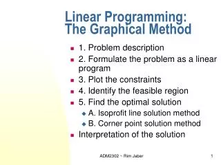
Example Problem No. 2 (1 of 3) Solve the following model graphically: Maximize Z = 4x1 + 5x2 subject to: x1 + 2x2 10 6x1 + 6x2 36 x1 4 x1, x2 0 Step 1: Plot the constraints as equations Figure 6.21 Constraint Equations Chapter 6 - Linear Programming: Model Formulation and Graphical Solution
Example Problem No. 2 (2 of 3) Maximize Z = 4x1 + 5x2 subject to: x1 + 2x2 10 6x1 + 6x2 36 x1 4 x1, x2 0 Step 2: Determine the feasible solution space Figure 6.22 Feasible Solution Space and Extreme Points Chapter 6 - Linear Programming: Model Formulation and Graphical Solution
Example Problem No. 2 (3 of 3) Maximize Z = 4x1 + 5x2 subject to: x1 + 2x2 10 6x1 + 6x2 36 x1 4 x1, x2 0 Step 3: Determine the corners; Step 4: Evaluate the objective function and identify the optimal solution. Figure 6.22 Optimal Solution Point Chapter 6 - Linear Programming: Model Formulation and Graphical Solution
Chapter 6 - Linear Programming: Model Formulation and Graphical Solution