Analysis of ecological data: "ecology isn't rocket science, it's harder” Kate Searle

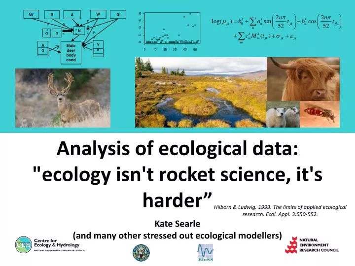
1. Gr W G E A PWTN PSN PEN PAN N σ σ PWTF Ye Analysis of ecological data: "ecology isn't rocket science, it's harder” Kate Searle (and many other stressed out ecological modellers) Ag Mule deer body cond Hilborn & Ludwig. 1993. The limits of applied ecological research. Ecol. Appl. 3:550-552.

2. Ecological processes and systems are multi-faceted and multi-scaled, such that an understanding of any individual part of the system requires recognition of drivers and constraints resulting from many interconnected processes Behaviour Spatial and temporal heterogeneity Populations Communities and Ecosystems

3. Moreover, states and variables within ecological systems are often not able to be measured directly, but must be inferred from surrogate observations. • It is often difficult to design experiments to adhere to standard statistical assumptions • This means that ecological data typically confound simple statistical approaches due to factors such as: • detectability • sampling or measurement error • unequal and irregular sampling effort over space and time How do we observe the animal we are interested in? How do we measure habitat quality for the animal?

4. Most common issues encountered: • Detectability– structural zeros, design error, observer error, animal error, naughty noughts (sampled outside habitat range) • Zero-inflated models, hurdle models • multi-state mark-recapture models • Hierarchical models – states and processes are measured at multiple scales • Spatial and temporal autocorrelation, or both Yi,t What we measured The “true” process Ei,t Hierarchical path analysis of the effect of habitat phenology on deer body condition Seasonal abundance models for Culicoides insects

5. Hierarchical path analysis of the effect of habitat phenology on deer body condition Asynchrony in vegetation phenology • spatially and temporally asynchronous pulses of plant growth • herbivores are able to prolong the period during which they have access to forage of peak nutritional value direct link to consumer fitness

6. PREDICTIONS: More asynchronous phenology = longer ‘green-up’ periods prolonged access = better winter body condition Shorter ‘green-up’ periods = compression in the time period over = poorer body condition Vegetation metrics: Integrative NDVI (INDVI):productivity and biomass – correlates well with ANPP. Higher INDVI = higher body condition. Maximal or mean slope of NDVI during green-up: fastness of greening up in the Spring – e.g., how elongated or compressed is the phenological development of plants in each individual’s home range. Elongated green-up – higher body condition. Onset of vegetation emergence: earlier vegetation onset = higher body condition.

7. DATA: • GPS location data, home ranges • NDVI • Climate • Data model for Mule deer body condition (% fat)

8. Error (exogenous independent variables) reflecting error in measurement or process variance σ Path coefficients for effect of e.g., N (NDVI) on F (%FAT) PNF Path analysis diagram for how performance (percent body fat) of mule deer is affected directly and indirectly by climate and plant phenologyin western Colorado. All lines in diagram represent a specific linear model. Green-up precipitation Winter precipitation Green-up temperature Elevation Aspect PWTN PWPN PSN PEN PAN PWPF NDVI indices σobs1 σ proc1 PWTF PNF Data model: Year Age PAF Mule deer body condition (percent fat) PYF Body fat measurement regression equation Capture month PRF PCF σ obs2 σ proc2 Range

9. Mean slope during vegetation green-up: Green-up precipitation Winter precipitation Green-up temperature Elevation Aspect 0.22 (0.13,0.30) 0.21 (0.14,0.30) -0.072 (-0.15,0.0037) -0.26 (-0.36,-0.16) 0.12 (0.013,0.22) Mean slope 0.049 (-0.041,0.14) -0.10 (-0.31,0.093) Mule deer body condition (percent fat) Mean slope adjusted R2: 0.28 BODY CONDITION adjusted R2: 0.62 Age -0.036 (-0.086,0.013) Path analysis diagram for how performance (percent fat) of adult, female mule deer is affected directly and indirectly by climate in western Colorado in 2008,2009 and 2010. Indirect linkages are manifested through a measure of the speed of vegetation green-up in the spring derived from NDVI measurements (‘mean slope’). All lines in the diagram represent a specific linear model. Thick solid lines represent strong evidence for an effect (95% credible interval does not overlap zero). Dotted lines represent no clear effect. Regression coefficient estimates are given with 95% credible intervals. ‘+’ predicted positive relationship, ‘-‘ predicted negative relationship.

10. Seasonal abundance models for Culicoides insects We know that the European distribution of Culicoidesdisease vectors is driven by climatic, host and land cover variation – how can we use phenology to better understand disease risk? Need to understand the spatial and temporal patterns of abundance C. pulicaris complex C. obsoletus complex C. dewulfi

11. Lots of zeros Orders of magnitude variation in abundance Messy

12. Modelling seasonal dynamics of Culiciodes spp. to generate vector abundance predictions for use in a BTV-1 spread model for the 2007 outbreak • 6 years of weekly trapping data from the whole of Spain • GLMM (Poisson –log link) with overdispersion, temporal autocorrelation (AR-1) and hierarchical structure for between site differences jth trap catch for site k (yjk) collected in week tjk: Seasonality in population with site-specific parameters Temporal autocorrelation Influence of meteorological parameters with site specific parameters overdispersion Corresponding meteorological variables:

13. and g is a fixed function; there appear to be two natural choices for g: • the triangular function g(w) = max(0, |1 − w|); or • the density function φ(w) of a standard normal distribution. λ : background midge abundance when not in a peak sk : width of peak (assumed to be the same for all sites, so s1 represents the longest peak and SK the shortest peak at each site) mik: magnitude of the k-thlongest peak at site i pik: timing of the k-th longest peak at site i φij : impact of time-varying covariates in modifying magnitude of the peak

14. Conclusions • Multi-site spatio-temporal models • extreme events – droughts and flood • detection of long-term trends in multifaceted variable times-series (sampling methods)

15. Thank you Adam Butler (BioSS) Beth Purse (CEH) Mindy Rice (Colorado Division of Wildlife) Tom Hobbs (Colorado State University) Simon Carpenter (Institute of Animal Health)