Download
1 / 27
270 likes | 423 Vues
Extensions of the Breeder’s Equation: Permanent Versus Transient Response Response to selection on the variance. µ. ∂. 2. 2. S. æ. æ. A. A. A. A. A. 2. R. =. h. S. +. +. +. ¢. ¢. ¢. +. æ. (. E. ;. E. ). +. æ. (. E. ;. E. ). s. i. r. e. o. d. a. m. o.

E N D
Extensions of the Breeder’s Equation: Permanent Versus Transient Response Response to selection on the variance
µ ∂ 2 2 S æ æ A A A A A 2 R = h S + + + ¢ ¢ ¢ + æ ( E ; E ) + æ ( E ; E ) s i r e o d a m o æ 2 2 4 z Breeder’s Equation Permanent component of response Response from epistasis Response from shared environmental effects Transient component of response --- contributes to short-term response. Decays away to zero over the long-term Permanent Versus Transient Response Considering epistasis and shared environmental values, the single-generation response follows from the midparent-offspring regression
µ ∂ 2 æ A A 2 R = S h + 2 2 æ z µ ∂ 2 æ ø A A 2 R ( 1 + ø ) = S h + ( 1 ° c ) 2 2 æ z Response with Epistasis The response after one generation of selection from an unselected base population with A x A epistasis is The contribution to response from this single generation after t generations of no selection is Response from additive effects (h2 S) is due to changes in allele frequencies and hence is permanent. Contribution from A x A due to linkage disequilibrium c is the average (pairwise) recombination between loci involved in A x A Contribution to response from epistasis decays to zero as linkage disequilibrium decays to zero
ø 2 R ( t + ø ) = t h S + ( 1 ° c ) R ( t ) A A RAA has a limiting value given by Time to equilibrium a function of c Why unselected base population? If history of previous selection, linkage disequilibrium may be present and the mean can change as the disequilibrium decays More generally, for t generation of selection followed by t generations of no selection (but recombination)
What about response with higher-order epistasis? Fixed incremental difference that decays when selection stops
Direct genetic effect on character G = A + D + I. E[A] = (Asire + Adam)/2 Maternal effect passed from dam to offspring is just A fraction m of the dam’s phenotypic value Maternal Effects: Falconer’s dilution model z = G + m zdam + e The presence of the maternal effects means that response is not necessarily linear and time lags can occur in response m can be negative --- results in the potential for a reversed response
A A d a m s i r e E ( z j A ; A ; z ) = + + m z o d a m s i r e d a m d a m 2 2 Regression of BV on phenotype A = π + b ( z ° π ) + e A A z z With no maternal effects, baz = h2 With maternal effects, a covariance between BV and maternal effect arises, with 2 æ = m æ = ( 2 ° m ) A ; M A The response thus becomes µ ∂ 2 2 h h ¢ π = S + m + S z d a m s i r e 2 ° m 2 ° m Parent-offspring regression under the dilution model In terms of parental breeding values, The resulting slope becomes bAz = h2 2/(2-m)
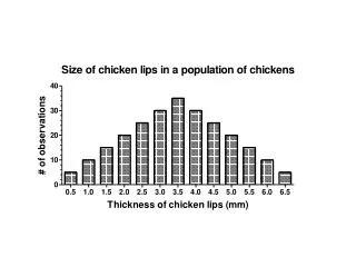
Recovery of genetic response after initial maternal correlation decays 0.10 0.05 0.00 Reversed response in 1st generation largely due to negative maternal correlation masking genetic gain -0.05 -0.10 -0.15 0 1 2 3 4 5 6 7 8 9 10 Response to a single generation of selection h2 = 0.11, m = -0.13 (litter size in mice) Cumulative Response to Selection (in terms of S) Generation
1.5 1.0 0.5 0.0 -0.5 -1.0 0 5 10 15 20 Selection occurs for 10 generations and then stops m = -0.25 m = -0.5 m = -0.75 Cumulative Response (in units of S) h2 = 0.35 Generation
For example, consider the response after 3 gens: Selection differential on great-grandparents Cov(offspring gen 3 on great-grandparents in gen 0) 8 great-grand parents from generation zero 2T-t = number of relatives from gen. t for offspring from gen T bT,t = cov(zT,zt) Ancestral Regressions When regressions on relatives are linear, we can think of the response as the sum over all previous contributions
Changes in the Variance under Selection The infinitesimal model --- each locus has a very small effect on the trait. Under the infinitesimal, require many generations for significant change in allele frequencies However, can have significant change in genetic variances due to selection creating linkage disequilibrium Under linkage equilibrium, freq(AB gamete) = freq(A)freq(B) With negative linkage disequilibrium, f(AB) < f(A)f(B), so that AB gametes are less frequent With positive linkage disequilibrium, f(AB) > f(A)f(B), so that AB gametes are more frequent
Additive variance Genic variance: value of Var(A) in the absence of disequilibrium function of allele frequencies Disequilibrium contribution. Requires covariances between allelic effects at different loci Additive variance with LD: Additive variance is the variance of the sum of allelic effects,
Selection-induced changes in d change s2A, s2z , h2 Dynamics of d: With unlinked loci, d loses half its value each generation (i.e, d in offspring is 1/2 d of their parents, Key: Under the infinitesimal model, no (selection-induced) changes in genic variance s2a
Consider the parent-offspring regression Change in variance from selection Dynamics of d: Computing the effect of selection in generating d Taking the variance of the offspring given the selected parents gives
+ = Recombination Selection In terms of change in d, At the selection-recombination equilibrium, Change in d = change from recombination plus change from selection This is the Bulmer Equation (Michael Bulmer), and it is akin to a breeder’s equation for the change in variance
=0.64 (43.9 - 52.7) = -3.2 4 2 e e e d = h ± ( æ ) z Application: Egg Weight in Ducks Rendel (1943) observed that while the change mean weight weight (in all vs. hatched) as negligible, but their was a significance decrease in the variance, suggesting stabilizing selection Before selection, variance = 52.7, reducing to 43.9 after selection. Heritability was h2 = 0.6 Var(A) = 0.6*52.7= 31.6. If selection stops, Var(A) is expected to increase to 31.6+3.2= 34.8 Var(z) should increase to 55.9, giving h2 = 0.62
Contribution of within- vs. between-family effects to Var(A) The total additive variance arises from two sources: differences between the mean BVs of families and variation of BVs within families When no LD is present, both these sources contribute equally, Var(A)/2. What happens when LD present? Consider parent-offspring regression in BA The within-family (or mendelian segregation variance) is simply the genic variance and is a constant (if allele frequencies not changing). LD is a function the between-family variance in BV When LD < 0, families are more similar than expected, When LD > 0, families are more dissimilar
Proportional reduction model: constant fraction k of variance removed Bulmer equation simplifies to Closed-form solution to equilibrium h2 Specific models of selection-induced changes in variances
Equilibrium h2 under direction truncation selection
Changes in the variance = changes in h2 and even S (under truncation selection) R(t) = h2(t) S(t)
In Class Problem You are selecting the upper 5% of a trait with h2 = 0.75 and sz2 = 100 initially in linkage equilibrium • Compute the response over 3 populations also compute d(t), h2(t), sz2(t), and S(t) • Compare the total 3 generations of response with the result from the standard breeder’s equation
Selection can also focus entirely on the variance (stabilizing & disruptive selection)
Disruptive selection inflates the variance after selection, generating positive d Stabilizing selection deflates the variance after selection, generating negative d
In class problem #2 You have a trait with phenotypic variance 100, heritability 0.4, d(0) = 0 Compare d, h2 and Var(A) after four generations of truncation selection (p=0.1) vs. double truncation selection (p=0.05 on both tails)