Download
1 / 35
360 likes | 686 Vues
Lecture 8B Frequency Response. Frequency Response. The most interesting type of system response Uses a sine wave forcing function input Interest is in the steady-state response instead of the transient response

E N D
Frequency Response • The most interesting type of system response • Uses a sine wave forcing function input • Interest is in the steady-state response instead of the transient response • Steady-state response to a step change only provides information about process gain • Transient response to sine wave change involves a fast change (gone within 4 Tp values) to consistent response oscillating at the input frequency
Attributes of Frequency Response • Two major characteristics of frequency response: • Output amplitude with respect to the input • Output phase lag or lead with respect to the input • Amplitude is attenuated or amplified depending on input frequency • Output oscillating out of phase withinput also depends on input frequency
First Order Frequency Response For a sine wave input to a first order process the output equals By partial fraction decomposition, numerators are:
First Order Frequency Response Now, by inverting back to the time domain: dies out as t increases Note: φis a function of Tpandω, but not of t. So for values of t/Tp≥ 4.0 (e-4 = 0.018), the process output , is a sine wave attenuated by whose value depends on ω being fast or slow.
First Order Frequency Response Attenuation and time shift between input and output sine waves (Kp=1). The phase angle φ of the output signal is calculated from φ = – 180*Δt/P, where Δt is the time shift and P is the period of oscillation.
Bodé Diagrams - for a First Order System Note that ωn = 1/Tp, the natural frequency of the system, so the X-axis is the relative frequency ω/ωn
Why is Frequency Response Analysis so Useful? • The amplitude ratio and phase lag provide info about system stability • These can be determined using the Laplace Transform directly to generate a Bodé Diagram • Can be used to study: • System identification (create a model) • Controller tuning • Stability of the control system • Robustness of the control system • Designing noise filters
Laplace and Complex Numbers Consider a complex number W defined as a + bj wherea represents the real part of W or Re(W) b represents the imaginary part of W or Im(W). Define the following terms to characterize this number in the complex domain (polar coordinates) The Modulus The Phase Angle
Laplace and Complex Numbers These two terms can be used to plot the complex number in a polar coordinate plane a = |W|cosθand b = |W|sinθ and W = |W|cosθ + j|W|sinθ
Laplace and Complex Numbers Since cosθ = (e+jθ + e-jθ)/2 and sinθ = (e+jθ – e-jθ)/2j Then W = |W|[(e+jθ + e-jθ)/2]+ j|W|[(e+jθ – e-jθ)/2j] W = |W|e+jθ Apply this complex knowledge to a First Order System: Substitute jω for s:
Laplace and Complex Numbers In polar coordinate form, this becomes: So by substituting jω for s and rearranging the transform into polar coordinate form, the amplitude ratio and phase angle for the system are obtained directly.
Second Order Frequency Response The original second order transform: Substitute jω for s:
Second Order Frequency Response In polar coordinate form, this becomes: So, steady state response is obtained directly for the second order system in a few steps and the Bodé Diagram can be plotted for different values of ωTp and ζ.
Bode Diagram - for Second Order System Note that ωn = 1/Tp, the natural frequency of the system, so the X-axis is the relative frequency ω/ωn
Notes on Second Order Frequency Response 2nd order response has maximum lag of 180° - twice a 1st order system. If phase angle exceeds 90°, then it is a higher order. The real problem faced by 2nd and higher order systems shows up at the natural frequency ωn . The amplitude ratio can be >>>> 1.0 and if ζapproaches0, the response is amplified to . With a 3rd order system, two critical frequencies may exist while for a 4th order system there can be three. Clearly such system responses are not desired or tolerable and must be avoided. As well the phase lag of higher order systems for high frequency inputs is equal to -90n where n is the system order. With such high lags, these systems are more difficult to control and design.
Bode Diagram for PI Controller • PI Controller
Bode Diagram for PI Controller • PI Controller with Kc = 2.0 and TI = 10
Bode Diagram for PD Controller • PD Controller
Bode Diagram for PD Controller • PD Controller with Kc = 2.0 and TD = 10
Bode Diagram for PID Controller • PID Controller
Bode Diagram for PD Controller • PID Controller with Kc = 2.0, TI = 10 and TD = 4
Notch filters are often used in control systems to eliminate the effects of mechanical resonance. The general transfer function for many types of filters, including notch filters, is equivalent to the transfer function of a PID controller.
Controller Design using Frequency Response • Advantages • Applicable to all orders & types of dynamic models • Designer can specify desired closed-loop response • Information on stability and sensitivity is obtained • Disadvantages • Approach is iterative and hence, is time-consuming–interactive computer graphics are necessary • Results often taken to be "gospel" (far from reality of most processes and plants) • Diagrams represent expected results for a model – not necessarily the real process
Frequency Response Stability Criteria Two principal methods to assess stability: - Bode Stability Criterion - Nyquist Stability Criterion The Bode Stability Criterion The Bode stability criterion states that a closed-loop system is unstable if the Frequency Response of the open-loop Transfer Function has an amplitude ratio greater than 1.0 at the critical frequency ωc. Otherwise the closed-loop system is stable. For the analysis, ωc is the value of ω where open-loop phase angle is -180°
Bode Stability Criteria • The Bode stability criterion • a closed-loop system is unstable if the Frequency Response of the open-loop Transfer Function has an amplitude ratio > 1.0 at the critical frequency Cω. • Otherwise the closed-loop system is stable. • Cωis where the open-loop phase angle = 180°
Bode Stability Criteria Example: • A process has a Transfer Function: • For proportional control, determine the closed-loop stability for three values of Kc = 1, 4, and 20.
Bode Stability Criteria Solution: • The Open Loop Transfer Function • The Bode plots for the three values of Kc are shown on the next slide. Note that the phase angle curves are identical for all three cases. (Explain?)
Bode Stability Criteria AROL φOL ωc ω/ωn
Ultimate Gain and Ultimate Period The Ultimate Controller Gain, KcU, is the maximum value of Kcthat results in stable closed loop system with proportional-only control (continuous oscillation). The Ultimate Period is the reciprocal of ωc as follows: KcUis determined from the Open Loop Frequency Response with P-only control and Kc =1. So:
Gain Margin GM is determined from the Amplitude Ratio Bodé Diagram. • Determine critical frequency (ωc) where phase lag = 180°. • Determine the value of the Amplitude Ratio (Ac) at ωc. • The Gain Margin is then defined as: GM = 1/Ac 4. The Bode Stability Criterion states: If the value of GM < 1.0, the system is stable for all input sine wave frequencies.
Phase Margin PM is determined from the Phase Lag Bodé Diagram. • Find the frequency ωgwhere the Amplitude Ratio= 1.0. • Determine the value of the phase lag φgat this ωg value • The phase margin is defined as PM = 180° + φg The Bode Stability Criterion states If PM is less than 0 , the system is stable for all sine wave input frequencies
Gain and Phase margin AROL ωg ωc ωc ω/ωn φg φOL ωg ωc ω/ωn
Gain Margin and Phase Margin 1.7 or 2.0 ≤ GM 30° or 45°≤ PM So, one can adjust Kc such that the GM is at least 1.7 or the PM must be more than 30°
Comparison of Transient Response • System response to a step change in set point for a PI controller tuned by frequency response ( ) and by Zeigler-Nichols rules ( ).