Download
1 / 18
180 likes | 297 Vues
Implementing Soak-Time Distribution Models in a GIS Framework. TERM PROJECT GIS in Water Resources (CE 394K.3) Fall 2000. Aruna Sivakumar Department of Civil Engineering (Transportation) University of Texas at Austin November 21 st 2000. Overview. Background – air quality modeling

E N D
Implementing Soak-Time Distribution Models in a GIS Framework TERM PROJECT GIS in Water Resources (CE 394K.3) Fall 2000 Aruna Sivakumar Department of Civil Engineering (Transportation) University of Texas at Austin November 21st 2000
Overview • Background – air quality modeling • Objective and Scope • TransCAD – GIS application • Modeling Background • Data & sources • Procedure • Results • Further work CE 394K.3 Fall 2000
Air Quality Modeling • Sources of air pollution – “criteria pollutants” CO, NO2, Pb, Ozone, SO2, PM10 • Clean Air Act (OAQPS) National Ambient Air Quality Standards (NAAQS) • Non-Attainmentand Conformity State Implementation Plan (SIP) Dallas-Fort Worth, TX Beaumont-Port Arthur Ozone Houston-Galveston-Brazoria El Paso Ozone, CO, PM10 CE 394K.3 Fall 2000
Mobile Emissions • Tailpipe Emissions a third of the air pollution in the country. TRAQ • Office of Transportation & Air Quality Vehicle & Engine Emissions Modeling Software MOBILE, PART5, Fuels Models, Non-Road models… • MOBILE –Highway vehicle emissions factor model • VOC (ozone), CO, NOx • 8 vehicle categories • 1952 to 2050 • ambient temp, avg traffic speeds, gasoline volatility CE 394K.3 Fall 2000
MOBILE6 (2000) • Inputs trip length estimates, trip start and trip ends, diurnal soak time, engine start soak time distributions, VMT by hour of day, facility, speed etc. • Outputs • “emission factors” expressed as grams of pollutant per vehicle mile traveled (g/mi). • Can be combined with estimates of total VMT • Emission type classes running, start, hot-soak, diurnal, resting, run loss, crankcase, refueling CE 394K.3 Fall 2000
Objective To implement the soak time distribution models in a GIS framework with the following features • user interactive input • output format suitable for MOBILE6 TransCAD + GISDK CE 394K.3 Fall 2000
TransCAD & GISDK Transportation GIS Software -better suited to application of statistical models -comprehensive sets of transportation, geographic and demographic data CE 394K.3 Fall 2000
-powerful development language (GISDK) for creating macros, add-ins, server applications, and custom front-ends -includes Caliper ScriptTMa macroprogramming language Execute Compile CE 394K.3 Fall 2000
Soak-time • Duration of time in which the vehicle’s engine is not operating and which precedes a successful vehicle start (i.e. one that does not result in a stall) • soak time < 12 hours HOT START • 70 soak time bins 1 – 30 min (1 min intervals) 30 – 60 min (2 min intervals) 60-720 min (30 min intervals) CE 394K.3 Fall 2000
Soak-time Models • Binary logit model – to estimate the fraction of first trip starts. • Log-linear soak-time models for first and non-first trip starts – to estimate the fraction of trip starts in each soak-time bin Soak Time depends on Time-of-day of trip start, activity purpose preceding the trip start, land use and demographic characteristics of the zone of trip start, trip characteristics CE 394K.3 Fall 2000
Inputs to MOBILE6 • fraction of trips in each of 70 soak-time bins by time-of-day and origin activity purpose (for each zone). Origin Activity Purpose Home Work School Social/Recreational Shopping Personal Business Other Time Periods Morning AM Peak AM Off Peak PM Off Peak PM Peak Evening
Data Dallas-Fort Worth 919 TAP Zones Zonal land use and Demographic characteristics Source: NCTCOG (North Central Texas Council of Govts.) GIS datafiles CE 394K.3 Fall 2000
Procedure • Import the D-FW shapefile into TransCAD Tap Zones: tap919.shp Attribute table for the TAP Zones
With the land-use and demographic data (from the attributes table) apply the soak time models in Excel • Create dataviews from the results in Excel, one for each time-period and link these to the corresponding zones. The soak-time distribution is now an attribute of the zone.
Attributes of selected zone Map Soak time distribution in the selected zone during the Morning period and by Origin activity purpose Soak time distributions by activity purpose
Results • A visual representation of the soak time distribution for each zone in the study area by time-of-day and origin activity purpose • Soak time distribution output data as inputs to MOBILE6 • First step in the development of a GIS-based user interface for emissions modeling
Further Work • Developing macros and add-ins using GISDK – user input interface, computation of soak time distribution, output files into MOBILE6