Download
1 / 39
390 likes | 559 Vues
q ij ~ N(y j , w j 2 ). Likelihood & Hierarchical Models. y j ~ N(m , t 2 ). This is an approximation…. Biased if n is small in many studies Biased if distribution of effect sizes isn't normal Biased for some estimators of w i. Solution: estimate t 2 from the data using Likelihood.

E N D
qij ~ N(yj,wj2) Likelihood & Hierarchical Models yj ~ N(m,t2)
This is an approximation… • Biased if n is small in many studies • Biased if distribution of effect sizes isn't normal • Biased for some estimators of wi
Likelihood: how well data support a given hypothesis. Note: Each and every parameter choice IS a hypothesis
L(θ|D) = p(D|θ) Where D is the data and θ is some choice of parameter values
Calculating a Likelihood m = 5, s = 1
Calculating a Likelihood m = 5, s = 1
Calculating a Likelihood m = 5, s = 1
Calculating a Likelihood m = 5, s = 1 L(m=5|D) = p(D|m=5) = y1*y2*y3 y1 y2 y3
The Maximum Likelihood Estimate is the value at which p(D|θ) is highest.
Calculating Two Likelihoods m = 3, s = 1 m = 7, s = 1
Calculating Two Likelihoods m = 3, s = 1 m = 7, s = 1
Calculating Two Likelihoods m = 3, s = 1 m = 7, s = 1
-2*Log-Likelihood = Deviance Ratio of deviances of nested models is ~ c2 Distributed, so, we can use it for tests!
Last Bits of Likelihood Review • θcan be as many parameters for as complex a model as we would like • Underlying likelihood equation also encompasses distributional information • Multiple algorithms for searching parameter space
rma(Hedges.D, Var.D, data=lep, method="ML") Random-Effects Model (k = 25; tau^2 estimator: DL) tau^2 (estimated amount of total heterogeneity): 0.0484 (SE = 0.0313) tau (square root of estimated tau^2 value): 0.2200 I^2 (total heterogeneity / total variability): 47.47% H^2 (total variability / sampling variability): 1.90 Test for Heterogeneity: Q(df = 24) = 45.6850, p-val = 0.0048 Model Results: estimate se zvalpvalci.lbci.ub 0.3433 0.0680 5.0459 <.0001 0.2100 0.4767
REML v. ML • In practice we use Restricted Maximum Likelihood (REML) • ML can produce biased estimates if multiple variance parameters are unknown • In practice, s2i from our studies is an observation. We must estimate s2i as well as t2
The REML Algorithm in a Nutshell • Set all parameters as constant, except one • Get the ML estimate for that parameter • Plug that in • Free up and estimate the next parameter • Plug that in • Etc... • Revisit the first parameter with the new values, and rinse and repeat
OK, so, we should use ML for random/mixed models – is that it?
Meta-Analytic Models so far • Fixed Effects: 1 grand mean • Can be modified by grouping, covariates • Random Effects: Distribution around grand mean • Can be modified by grouping, covariates • Mixed Models: • Both predictors and random intercepts
Hierarchical Models • Study-level random effect • Study-level variation in coefficients • Covariates at experiment and study level
Hierarchical Models • Random variation within study (j) and between studies (i) Tij ~ N(qij, sij2) qij ~ N(yj,wj2) yj ~ N(m,t2)
Hierarchical Partitioning of One Study Study Mean Variation due to w Variation due to t Grand Mean
Hierarchical Models in Paractice • Different methods of estimation • We can begin to account for complex non-independence • But for now, we'll start simple…
Linear Mixed Effects Model > marine_lme <- lme(LR ~ 1, random=~1|Study/Entry, data=marine, weights=varFunc(~VLR))
summary(marine_lme) ... Random effects: Formula: ~1 | Study (Intercept) StdDev: 0.2549197 Formula: ~1 | Entry %in% Study (Intercept) Residual StdDev: 0.02565482 2.172048 ... t w
summary(marine_lme) ... Variance function: Structure: fixed weights Formula: ~VLR Fixed effects: LR ~ 1 Value Std.Error DF t-value p-value (Intercept) 0.1807378 0.05519541 106 3.274508 0.0014 ...
Meta-Analytic Version > marine_mv <- rma.mv(LR ~ 1, VLR, data=marine, random= list(~1|Study, ~1|Entry)) Allows greater flexibility in variance structure and correlation, but, some under-the-hood differences
summary(marine_mv) Multivariate Meta-Analysis Model (k = 142; method: REML) logLik Deviance AIC BIC AICc -126.8133 253.6265 259.6265 268.4728 259.8017 Variance Components: estimsqrtnlvls fixed factor sigma^2.1 0.1731 0.4160 142 no Entry sigma^2.2 0.0743 0.2725 36 no Study w2 t2
summary(marine_mv) Test for Heterogeneity: Q(df = 141) = 1102.7360, p-val < .0001 Model Results: estimate se zvalpvalci.lbci.ub 0.1557 0.0604 2.5790 0.0099 0.0374 0.2741 ** --- Signif. codes: 0 ‘***’ 0.001 ‘**’ 0.01 ‘*’ 0.05 ‘.’ 0.1 ‘ ’ 1
Comparison of lme and rma.mv • lme and rma.mv use different weighting • rma.mvassumes variance is known • lmeassumes you know proportional differences in variance http://www.metafor-project.org/doku.php/tips:rma_vs_lm_and_lme