Download

1 / 124
1.26k likes | 1.58k Vues
SKEMA Ph.D programme 2010-2011. Class 6 Qualitative Dependent Variable Models. Lionel Nesta Observatoire Français des Conjonctures Economiques Lionel.nesta@ofce.sciences-po.fr. Structure of the class. The linear probability model Maximum likelihood estimations

E N D
SKEMA Ph.D programme 2010-2011 Class 6Qualitative Dependent Variable Models Lionel Nesta Observatoire Français des Conjonctures Economiques Lionel.nesta@ofce.sciences-po.fr
Structure of the class • The linear probability model • Maximum likelihood estimations • Binary logit models and some other models • Multinomial models • Ordered multinomial models • Count data models
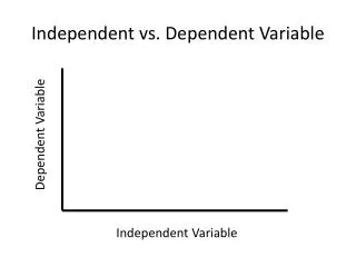
The linear probability model • When the dependent variable is binary (0/1, for example, Y=1 if the firm innovates, 0 otherwise), OLS is called the linear probability model. • How should one interpret βj? Provided that OLS4 – E(u|X)=0 – holds true, then:
The linear probability model • Y follows a Bernoulli distribution with expected value P. This model is called the linear probability model because its expected value, conditional on X, and written E(Y|X), can be interpreted as the conditional probability of the occurrence of Y given values of X. • β measures the variation of the probability of success for a one-unit variation of X (ΔX=1)
Limits of the linear probability model (1) Non normality of errors • OLS6 : The error term is independent of all RHS and follows a normal distribution with zero mean and variance σ² • Since the errors are the complement to unity of the conditional probability, they follow a Bernoulli distribution, not a normal distribution.
Limits of the linear probability model (1) Non normality of errors
Limits of the linear probability model (2) Heteroskedastic errors • OLS5 : The variance of the error term, u, conditional on RHS, is the same for all values of RHS • The error term is itself distributed Bernoulli, and its variance depends on X. Hence it is heteroskedastic
Limits of the linear probability model (2) Heteroskedastic errors
Limits of the linear probability model (3) Fallacious predictions • By definition, a probability is always in the unit interval [0;1] • But OLS does not guarantee this condition • Predictions may lie outside the bound [0;1] • The marginal effect is constant , since P = E(Y|X) grows linearly with X. This is not very realistic (ex: the probability to give birth conditional on the number of children already born)
Fallacious predictions Limits of the linear probability model (3) Fallacious predictions
Limits of the linear probability model (4) A downward bias in the coefficient of determination R² • Observed values are 1 or 0, whereas predictions should lie between 0 and 1: [0;1]. • Comparing predicted with observed variables, the goodness of fit as assessed by the R² is systematically low .
Fallacious predictions which lower the R2 Limits of the linear probability model (4) Fallacious predictions
Limits of the linear probability model (4) • Non normality of errors • Heteroskedastic errors • Fallacious predictions • A downward bias in the R²
Overcoming the limits of the LPM • Non normality of errors • Increase sample size • Heteroskedastic errors • Use robust estimators • Fallacious prediction • Perform non linear or constrained regressions • A downward bias in the R² • Do not use it as a measure of goodness of fit
Persistent use of LPM • Although it has limits, the LPM is still used • In the process of data exploration (early stages of the research) • It is a good indicator of the marginal effect of the representative observation (at the mean) • When dealing with very large samples, least squares can overcome the complications imposed by maximum likelihood techniques. • Time of computation • Endogeneity and panel data problems
Probability, odds and logit • We need to explain the occurrence of an event: the LHS variable takes two values : y={0;1}. • In fact, we need to explain the probability of occurrence of the event, conditional on X: P(Y=y | X) ∈ [0 ; 1]. • OLS estimations are not adequate, because predictions can lie outside the interval [0 ; 1]. • We need to transform a real number, say z to ∈ ]-∞;+∞[ into P(Y=y | X) ∈ [0 ; 1]. • The logistic transformation links a real number z ∈ ]-∞;+∞[ to P(Y=y | X) ∈ [0 ; 1].It is also called the link function
The logit link function Let us make sure that the transformation of z lies between 0 and1
The logit model Hence the probability of any event to occur is : But what is z?
The odds ratio The odds ratio is defined as the ratio of the probability and its complement. Taking the log yields z. Hence z is the log transform of the odds ratio. • This has two important characteristics : • Z ∈ ]-∞;+∞[ and P(Y=1) ∈ [0 ; 1] • The probability is not linear in z (The plot linking z with straight line)
The logit transformation • The preceding table matches levels of probability with the odds ratio. • The probability varies between 0 and 1, The odds varies between 0 and + ∞. The log of the odds varies between – ∞ and + ∞ . • Notice that the distribution of the log of the odds is symetrical.
The logit link function The whole trick that can overcome the OLS problem is then to posit: But how can we estimate the above equation knowing that we do not observe z?
Maximum likelihood estimations • OLS can be of much help. We will use Maximum Likelihood Estimation (MLE) instead. • MLE is an alternative to OLS. It consists of finding the parameters values which is the most consistent with the data we have. • In Statistics, the likelihood is defined as the joint probability to observe a given sample, given the parameters involved in the generating function. • One way to distinguish between OLS and MLE is as follows: OLS adapts the model to the data you have : you only have one model derived from your data. MLE instead supposes there is an infinity of models, and chooses the model most likely to explain your data.
Likelihood functions • Let us assume that you have a sample of n random observations. Let f(yi) be the probability that yi = 1 or yi = 0. The joint probability to observe jointly n values of yiis given by the likelihood function: • We need to specify function f(.). It comes from the empirical descrite distribution of an event that can have only two outcome : a success (yi = 1) or a failure (yi = 0). This is the binomial distribution. Hence:
Likelihood functions • Knowing p (as the logit), having defined f(.), we come up with the likelihood function:
Log likelihood (LL) functions • The log transform of the likelihood function (the log likelihood) is much easier to manipulate, and is written:
Maximum likelihood estimations • The LL function can yield an infinity of values for the parameters β. • Given the functional form of f(.)and the n observations at hand, which values of parameters β maximize the likelihood of my sample? • In other words, what are the most likely values of my unknown parameters β given the sample I have?
Maximum likelihood estimations The LL is globally concave and has a maximum. The gradient is used to compute the parameters of interest, and the hessian is used to compute the variance-covariance matrix. However, there is not analytical solutions to this non linear problem. Instead, we rely on a optimization algorithm (Newton-Raphson) You need to imagine that the computer is going to generate all possible values of β, and is going to compute a likelihood value for each (vector of ) values to then choose (the vector of) β such that the likelihood is highest.
Example: Binary Dependent Variable We want to explore the factors affecting the probability of being successful innovator (inno = 1): Why? 352 (81.7%) innovate and 79 (18.3%) do not. The odds of carrying out a successful innovation is about 4 against 1 (as 352/79=4.45). The log of the odds is 1.494 (z = 1.494) For the sample (and the population?) of firms the probability of being innovative is four times higher than the probability of NOT being innovative
Logistic Regression with STATA Instruction Stata : logit logit y x1 x2 x3 … xk [if] [weight] [, options] • Options • noconstant : estimates the model without the constant • robust : estimates robust variances, also in case of heteroscedasticity • if : it allows to select the observations we want to include in the analysis • weight : it allows to weight different observations
Let’s start and run a constant only model logit inno Logistic Regression with STATA Goodness of fit Parameter estimates, Standard errors and z values
What does this simple model tell us ? Remember that we need to use the logit formula to transform the logit into a probability : Interpretation of Coefficients
The constant 1.491 must be interpreted as the log of the odds ratio. Using the logit link function, the average probability to innovate is dis exp(_b[_cons])/(1+exp(_b[_cons])) We find exactly the empirical sample value: 81,7% Interpretation of Coefficients
A positive coefficient indicates that the probability of innovation success increases with the corresponding explanatory variable. A negative coefficient implies that the probability to innovate decreases with the corresponding explanatory variable. Warning! One of the problems encountered in interpreting probabilities is their non-linearity: the probabilities do not vary in the same way according to the level of regressors This is the reason why it is normal in practice to calculate the probability of (the event occurring) at the average point of the sample Interpretation of Coefficients
Interpretation of Coefficients • Let’s run the more complete model • logit inno lrdilassetsspe biotech
Interpretation of Coefficients • Using the sample mean values of rdi, lassets, spe andbiotech, we compute the conditional probability :
Marginal Effects • It is often useful to know the marginal effect of a regressor on the probability that the event occur (innovation) • As the probability is a non-linear function of explanatory variables, the change in probability due to a change in one of the explanatory variables is not identical if the other variables are at the average, median or first quartile, etc. level. • prvalue provides the predicted probabilities of a logit model (or any other) • prvalue • prvalue , x(lassets=10) rest(mean) • prvalue , x(lassets=11) rest(mean) • prvalue , x(lassets=12) rest(mean) • prvalue , x(lassets=10) rest(median) • prvalue , x(lassets=11) rest(median) • prvalue , x(lassets=12) rest(median)
Marginal Effects • prchange provides the marginal effect of each of the explanatory variables for the majority of the variations of the desired values • prchange [varlist] [if] [in range] ,x(variables_and_values) rest(stat) fromto • prchange • prchange, fromto • prchange , fromto x(size=10.5) rest(mean)
Goodness of Fit Measures • In ML estimations, there is no such measure as the R2 • But the log likelihood measure can be used to assess the goodness of fit. But note the following : • The higher the number of observations, the lower the joint probability, the more the LL measures goes towards -∞ • Given the number of observations, the better the fit, the higher the LL measures (since it is always negative, the closer to zero it is) • The philosophy is to compare two models looking at their LL values. One is meant to be the constrained model, the other one is the unconstrained model.
Goodness of Fit Measures • A model is said to be constrained when the observed set the parameters associated with some variable to zero. • A model is said to be unconstrained when the observer release this assumption and allows the parameters associated with some variable to be different from zero. • For example, we can compare two models, one with no explanatory variables, one with all our explanatory variables. The one with no explanatory variables implicitly assume that all parameters are equal to zero. Hence it is the constrained model because we (implicitly) constrain the parameters to be nil.
The likelihood ratio test (LR test) • The most used measure of goodness of fit in ML estimations is the likelihood ratio. The likelihood ratio is the difference between the unconstrained model and the constrained model. This difference is distributed c2. • If the difference in the LL values is (no) important, it is because the set of explanatory variables brings in (un)significant information. The null hypothesis H0is that the model brings no significant information as follows: • High LR values will lead the observer to reject hypothesis H0and accept the alternative hypothesis Hathat the set of explanatory variables does significantly explain the outcome.
The McFadden Pseudo R2 • We also use the McFadden Pseudo R2(1973). Its interpretation is analogous to the OLS R2. However its is biased doward and remain generally low. • Le pseudo-R2also compares The likelihood ratio is the difference between the unconstrained model and the constrained model and is comprised between 0 and 1.
Goodness of Fit Measures Constrained model Unconstrained model
Other usage of the LR test • The LR test can also be generalized to compare any two models, the unconstrained one being nested in the constrained one. • Any variable which is added to a model can be tested for its explanatory power as follows : • logit [modèle contraint] • est store [nom1] • logit [modèle non contraint] • est store [nom2] • lrtest nom2 nom1
Goodness of Fit Measures LR test on the added variable (biotech)
Quality of predictions • Lastly, one can compare the quality of the prediction with the observed outcome variable (dummy variable). • One must assume that when the probability is higher than 0.5, then the prediction is that the vent will occur (most likely • And then one can compare how good the prediction is as compared with the actual outcome variable. • STATA does this for us: • estat class