Download
1 / 39

E N D
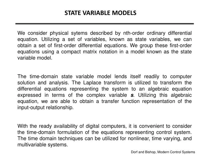
STATE VARIABLE MODELS We consider physical sytems described by nth-order ordinary differential equation. Utilizing a set of variables, known as state variables, we can obtain a set of first-order differential equations. We group these first-order equations using a compact matrix notation in a model known as the state variable model. The time-domain state variable model lends itself readily to computer solution and analysis. The Laplace transform is utilized to transform the differential equations representing the system to an algebraic equation expressed in terms of the complex variable s. Utilizing this algebraic equation, we are able to obtain a transfer function representation of the input-output relationship. With the ready availability of digital computers, it is convenient to consider the time-domain formulation of the equations representing control system. The time domain techniques can be utilized for nonlinear, time varying, and multivariable systems. Dorf and Bishop, Modern Control Systems
A time-varying control system is a system for which one or more of the parameters of the system may vary as a function of time. For example, the mass of a missile varies as a function of time as the fuel is expended during flight. A multivariable system is a system with several input and output. The State Variables of a Dynamic System: The time-domain analysis and design of control systems utilizes the concept of the state of a system. The state of a system is a set of variables such that the knowledge of these variables and the input functions will, with the equations describing the dynamics, provide the future state and output of the system.
x(0) Initial conditions Input Signals Output Signals u1(t) System u(t) System y(t) u2(t) Input Output For a dynamic system, the state of a system is described in terms of a set of state variables The state variables are those variables that determine the future behavior of a system when the present state of the system and the excitation signals are known. Consider the system shown in Figure 1, where y1(t) and y2(t) are the output signals and u1(t) and u2(t) are the input signals. A set of state variables [x1 x2 ... xn] for the system shown in the figure is a set such that knowledge of the initial values of the state variables [x1(t0) x2(t0) ... xn(t0)] at the initial time t0, and of the input signals u1(t) and u2(t) for t˃=t0, suffices to determine the future values of the outputs and state variables. y1(t) y2(t) Figure 1. Dynamic system.
k c m y(t) u(t) The state variables describe the future response of a system, given the present state, the excitation inputs, and the equations describing the dynamics. A simple example of a state variable is the state of an on-off light switch. The switch can be in either the on or the off position, and thus the state of the switch can assume one of two possible values. Thus, if we know the present state (position) of the switch at t0 and if an input is applied, we are able to determine the future value of the state of the element. The concept of a set of state variables that represent a dynamic system can be illustrated in terms of the spring-mass-damper system shown in Figure 2. The number of state variables chosen to represent this system should be as small as possible in order to avoid redundant state variables. A set of state variables sufficient to describe this system includes the position and the velocity of the mass. Figure 2. 1-dof system.
Therefore we will define a set of variables as [x1 x2], where Kinetic and Potential energies, virtual work. Lagrangian of the system is expressed as Generalized Force Lagrange’s equation Equation of motion in terms of state variables. We can write the equations that describe the behavior of the spring-mass-damper system as the set of two first-order differential equations.
iL ic L u(t) R Vo Vc C Current source This set of difefrential equations describes the behavior of the state of the system in terms of the rate of change of each state variables. As another example of the state variable characterization of a system, consider the RLC circuit shown in Figure 3. The state of this system can be described in terms of a set of variables [x1 x2], where x1 is the capacitor voltage vc(t) and x2 is equal to the inductor current iL(t). This choice of state variables is intuitively satisfactory because the stored energy of the network can be described in terms of these variables. Figure 3
Therefore x1(t0) and x2(t0) represent the total initial energy of the network and thus the state of the system at t=t0. Utilizing Kirchhoff’s current low at the junction, we obtain a first order differential equation by describing the rate of change of capacitor voltage Kirchhoff’s voltage low for the right-hand loop provides the equation describing the rate of change of inducator current as The output of the system is represented by the linear algebraic equation Dorf and Bishop, Modern Control Systems
We can write the equations as a set of two first order differential equations in terms of the state variables x1 [vC(t)] and x2 [iL(t)] as follows: The output signal is then Utilizing the first-order differential equations and the initial conditions of the network represented by [x1(t0) x2(t0)], we can determine the system’s future and its output. The state variables that describe a system are not a unique set, and several alternative sets of state variables can be chosen. For the RLC circuit, we might choose the set of state variables as the two voltages, vC(t) and vL(t).
In an actual system, there are several choices of a set of state variables that specify the energy stored in a system and therefore adequately describe the dynamics of the system. The state variables of a system characterize the dynamic behavior of a system. The engineer’s interest is primarily in physical, where the variables are voltages, currents, velocities, positions, pressures, temperatures, and similar physical variables. The State Differential Equation: The state of a system is described by the set of first-order differential equations written in terms of the state variables [x1 x2 ... xn]. These first-order differential equations can be written in general form as
Thus, this set of simultaneous differential equations can be written in matrix form as follows: n: number of state variables, m: number of inputs. The column matrix consisting of the state variables is called the state vector and is written as Dorf and Bishop, Modern Control Systems
The vector of input signals is defined as u. Then the system can be represented by the compact notation of the state differential equation as This differential equation is also commonly called the state equation. The matrix A is an nxn square matrix, and B is an nxm matrix. The state differential equation relates the rate of change of the state of the system to the state of the system and the input signals. In general, the outputs of a linear system can be related to the state variables and the input signals by the output equation Where y is the set of output signals expressed in column vector form. The state-space representation (or state-variable representation) is comprised of the state variable differential equation and the output equation.
We can write the state variable differential equation for the RLC circuit as and the output as The solution of the state differential equation can be obtained in a manner similar to the approach we utilize for solving a first order differential equation. Consider the first-order differential equation Where x(t) and u(t) are scalar functions of time. We expect an exponential solution of the form eat. Taking the Laplace transform of both sides, we have
therefore, The inverse Laplace transform of X(s) results in the solution We expect the solution of the state differential equation to be similar to x(t) and to be of differential form. The matrix exponential function is defined as Dorf and Bishop, Modern Control Systems
which converges for all finite t and any A. Then the solution of the state differential equation is found to be where we note that [sI-A]-1=ϕ(s), which is the Laplace transform of ϕ(t)=eAt. The matrix exponential function ϕ(t) describes the unforced response of the system and is called the fundamental or state transitionmatrix. Dorf and Bishop, Modern Control Systems
THE TRANSFER FUNCTION FROM THE STATE EQUATION The transfer function of a single input-single output (SISO) system can be obtained from the state variable equations. where y is the single output and u is the single input. The Laplace transform of the equations where B is an nx1 matrix, since u is a single input. We do not include initial conditions, since we seek the transfer function. Reordering the equation
Therefore, the transfer function G(s)=Y(s)/U(s) is Example: Determine the transfer function G(s)=Y(s)/U(s) for the RLC circuit as described by the state differential function
Then the transfer function is Dorf and Bishop, Modern Control Systems
State-space object sys_ss=ss(sys_tf) sys_tf=tf(sys_ss) sys=ss(A,B,C,D) The ss function Figure 4. ANALYSIS OF STATE VARIABLE MODELS USING MATLAB Given a transfer function, we can obtain an equivalent state-space representation and vice versa. The function tf can be used to convert a state-space representation to a transfer function representation; the function ss can be used to convert a transfer function representation to a state-space representation. The functions are shown in Figure 4, where sys_tf represents a transfer function model and sys_ss is a state space representation. Linear system model conversion Dorf and Bishop, Modern Control Systems
For instance, consider the third-order system We can obtain a state-space representation using the ss function. The state-space representation of the system given by G(s) is Matlab code Transfer function: 2 s^2 + 8 s + 6 ---------------------- s^3 + 8 s^2 + 16 s + 6 a = x1 x2 x3 x1 -8 -4 -1.5 x2 4 0 0 x3 0 1 0 b = u1 x1 2 x2 0 x3 0 c = x1 x2 x3 y1 1 1 0.75 d = u1 y1 0 Continuous-time model. num=[2 8 6];den=[1 8 16 6]; sys_tf=tf(num,den) sys_ss=ss(sys_tf) Answer
1 1 1 Y(s) R(s) R(s) x3 x1 4 x2 1 1/s 1/s 0.75 1/s 1/s 1/s 2 2 -8 -8 -4 -1.5 Block diagram with x1 defined as the leftmost state variable.
We can use the function expm to compute the transition matrix for a given time. The expm(A) function computes the matrix exponential. By contrast the exp(A) function calculates eaij for each of the elements aijϵA. For the RLC network, the state-space representation is given as: The initial conditions are x1(0)=x2(0)=1 and the input u(t)=0. At t=0.2, the state transition matrix is calculated as Phi = 0.9671 -0.2968 0.1484 0.5219 >>A=[0 -2;1 -3], dt=0.2; Phi=expm(A*dt)
System u(t) y(t) Output Arbitrary Input t=times at which response is computed t y(t)=output response at t T: time vector X(t)=state response at t t Initial conditions (optional) u=input [y,T,x]=lsim(sys,u,t,x0) The state at t=0.2 is predicted by the state transition method to be The time response of a system can also be obtained by using lsim function. The lsim function can accept as input nonzero initial conditions as well as an input function. Using lsim function, we can calculate the response for the RLC network as shown below. Dorf and Bishop, Modern Control Systems
Matlab code u=0*t clc;clear A=[0 -2;1 -3];B=[2;0];C=[1 0];D=[0]; sys=ss(A,B,C,D) %state-space model x0=[1 1]; %initial conditions t=[0:0.01:1]; u=0*t; %zero input [y,T,x]=lsim(sys,u,t,x0); subplot(211),plot(T,x(:,1)) xlabel('Time (seconds)'),ylabel('X_1') subplot(212),plot(T,x(:,2)) xlabel('Time (seconds)'),ylabel('X_2') u=3*t u=3*exp(-2*t)
y(t) q(t) y(t) Head mass u(t) Force Motor mass u(t) M=M1+M2 Head position M1 M2 b1 b2 b1 Figure 5b Figure 5a Example: Dorf and Bishop, Modern Control Systems, p173. Consider the head mount of a disk reader shown in the figure. We will attempt to derive a model for the system shown in Figure 5a. Here we identify the motor mass M1 and the head mount mass as M2. The flexure spring is represented by the spring constant k. The force u(t) to drive the mass M1 is generated by the DC motor. If the spring is absolutely rigid (nonspringy), then we obtain the simplifed model shown in Figure 5b. Typical parameters for the two-mass system are given in Table 1. Table 1. Typical parameters of the two-mass model Motor mass M1= 0.02 kg Friction at mass 1 b1=410x10-3 kgs/m Motor constant Km=0.1025 Nm/A Flexure spring 10<=k<=inf Field resistance R=1 Ω Friction at mass 2 b2=4.1x10⁻³ kgm/s Head mounting M2=0.0005 kg Field inductance L=1 mH Head position y(t)=x2(t)
To develop a state variable model, we choose the state variables as x1=q and x2=y. Then we have Motor coil Two-mass system V(s) U(s) Force In matrix form, Note that the output is dy/dt=x4.Also, for L=0 or negligible inductance, then u(t)=Kmv(t). For the typical parameters and k=10, we have
clc;clear k=10; M1=0.02;M2=0.0005; b1=410e-3;b2=4.1e-3; t=0:0.001:1.5; A=[0 0 1 0;0 0 0 1;-k/M1 k/M1 -b1/M1 0;k/M2 -k/M2 0 -b2/M2]; B=[0;0;1/M1;0];C=[0 0 0 1];D=[0]; sys=ss(A,B,C,D) y=step(sys,t); plot(t,y);grid xlabel('Time (seconds)'),ylabel('ydot (m/s)') Velocity of Mass 2 (Head) k=10 N/m Dorf and Bishop, Modern Control Systems
k=1000 N/m k=100 N/m k=100000 N/m
THE DESIGN OF STATE VARIABLE FEEDBACK SYSTEMS The time-domain method, expressed in terms of state variables, can also be utilized to design a suitable compensation scheme for a control system. Typically, we are interested in controlling the system with a control signal, u(t), which is a function of several measurable state variables. Then we develop a state variable controller that operates on the information available in measured form. State variable design is typically comprised of three steps. In the first step, we assume that all the state variables are measurable and utilize them in a full-state feedback control law. Full-state feedback is not usually practical because it is not possible (in general) to measure all the states. In paractice, only certain states (or linear combinations thereof) are measured and provided as system outputs. The second step in state varaible design is to construct an observer to estimate the states that are not directly sensed and available as outputs. Observers can either be full-state observers or reduced-order observers. Reduced-order observers account for the fact that certain states are already available as system outputs; hence they do not need to be estimated. The final step in the design process is to appropriately connect the observer to the full-state feedback conrol low. It is common to refer to the state-varaible controller as a compensator. Additionally, it is possible to consider reference inputs to the state variable compensator to complete the design. Dorf and Bishop, Modern Control Systems
CONTROLLABILITY: Full-state feedback design commonly relies on pole-placement techniques. It is important to note that a system must be completely controllable and completely observable to allow the flexibility to place all the closed-loop system poles arbitrarily. The concepts of controllability and observability were introduced by Kalman in the 1960s. A system is completely controllable if there exists an unconstrained control u(t) that can transfer any initial state x(t0) to any other desired location x(t) in a finite time, t0≤t≤T.
For the system we can determine whether the system is controllable by examining the algebraic condition The matrix A is an nxn matrix an B is an nx1 matrix. For multi input systems, B can be nxm, where m is the number of inputs. For a single-input, single-output system, the controllability matrix Pc is described in terms of A and B as which is nxn matrix. Therefore, if the determinant of Pc is nonzero, the system is controllable.
Example: Consider the system The determinant of Pc =1 and ≠0 , hence this system is controllable.
Example. Consider a system represented by the two state equations The output of the system is y=x2. Determine the condition of controllability. The determinant of pc is equal to d, which is nonzero only when d is nonzero. Dorf and Bishop, Modern Control Systems
The controllability matrix Pc can be constructed in Matlab by using ctrb command. From two-mass system, Pc = 1.0e+007 * 0 0.0000 -0.0001 -0.0004 0 0 0 0.1000 0.0000 -0.0001 -0.0004 0.0594 0 0 0.1000 -2.8700 rank_Pc = 4 det_Pc = -2.5000e+015 clc clear A=[0 0 1 0;0 0 0 1;-500 500 -20.5 0;20000 -20000 0 -8.2]; B=[0;0;50;0]; Pc=ctrb(A,B) rank_Pc=rank(Pc) det_Pc=det(Pc) The system is controllable.
OBSERVABILITY: All the poles of the closed-loop system can be placed arbitrarily in the complex plane if and only if the system is observable and controllable. Observability refers to the ability to estimate a state variable. A system is completely observable if and only if there exists a finite time T such that the initial state x(0) can be determined from the observation history y(t) given the control u(t). Consider the single-input, single-output system where C is a 1xn row vector, and x is an nx1 column vector. This system is completely observable when the determinant of the observability matrix P0 is nonzero.
The observability matrix, which is an nxn matrix, is written as Example: Consider the previously given system Dorf and Bishop, Modern Control Systems
Thus, we obtain The det P0=1, and the system is completely observable. Note that determination of observability does not utility the B and C matrices. Example: Consider the system given by
We can check the system controllability and observability using the Pc and P0 matrices. From the system definition, we obtain Therefore, the controllability matrix is determined to be Therefore, the controllability matrix is determined to be det Pc=0 and rank(Pc)=1. Thus, the system is not controllable. Dorf and Bishop, Modern Control Systems
From the system definition, we obtain Therefore, the observability matrix is determined to be det PO=0 and rank(PO)=1. Thus, the system is not observable. If we look again at the state model, we note that However,
Thus, the system state variables do not depend on u, and the system is not controllable. Similarly, the output (x1+x2) depends on x1(0) plus x2(0) and does not allow us to determine x1(0) and x2(0) independently. Consequently, the system is not observable. The observability matrix PO can be constructed in Matlab by using obsv command. From two-mass system, Po = 1 1 1 1 rank_Po = 1 det_Po = 0 clc clear A=[2 0;-1 1]; C=[1 1]; Po=obsv(A,C) rank_Po=rank(Po) det_Po=det(Po) The system is not observable. Dorf and Bishop, Modern Control Systems