Download
1 / 21
210 likes | 212 Vues
MHD Coronal Seismology with SDO/AIA UK Community Views Len Culhane, MSSL with inputs from Valery Nakariakov, Warwick Ineke de Moortel, St Andrews David Williams, MSSL Mihalis Mathioudakis, Queen’s University. 1. Transverse (Kink) Oscillations. Commonly accepted interpretation

E N D
MHD Coronal Seismology with SDO/AIAUK Community ViewsLen Culhane, MSSLwith inputs fromValery Nakariakov, WarwickIneke de Moortel, St AndrewsDavid Williams, MSSLMihalis Mathioudakis, Queen’s University
1. Transverse (Kink) Oscillations Commonly accepted interpretation • Standing fast magnetoacoustic m=1 modes of coronal loops Seismological applications • Estimation of the mean value of the magnetic field strength (Nakariakov and Ofman, 2001) • Estimation of the density stratification in the loop (Andries et al. 2005) Open questions • Excitation Mechanisms • Decay Mechanisms • Selectivity of the Excitation • Role of Nonlinear Effects • Use of Observations for Seismology
Necessary Theoretical Developments • 3- D MHD modelling • Incorporation of fine structuring effects • - stratification, curvature, nonlinearity in simple • magnetic geometries (isolated loop, arcade, • parallel loops bundle) • Parametric numerical study of the dependence of • observables on model parameters (period, decay • time, time dependence, scaling laws) • Derivation of simple analytical expressions • Linking the observables with physical parameters in the loop (e.g. magnetic • field strength) • 3- D MHD numerical modelling in extrapolated magnetic geometry • Linking the outcomes with analytical theory • Testing the robustness of the modelling, in particular to the errors in extrapolation • and to computational constraints • Creation of seismological methods for the determination of coronal currents by • MHD waves
2. Longitudinal (Slow) Waves Commonly Accepted Interpretation: • Slow magnetoacoustic perturbations, guided by magnetic field lines. Seismological Applications: • Observables (periods, wave lengths, height evolution) depend strongly upon thermal effects - information about the heating function. • Modes are natural probes of coronal thermal structure - simultaneous detection of mode in TRACE 171A and 195A suggested as a probe of sub-resolution structuring of the corona (King et al., 2003) Open Questions: • What is their origin and driver? • What determines the periodicity and coherence of propagating waves? • What is the physical mechanism for the abrupt disappearance of the waves at a certain height • Are the waves connected with the running penumbra waves? (King et al., 2003)
Necessary Theoretical Developments • Effects of transverse structuring (physical and observational). • Incorporation of a realistic TR and chromosphere in the model, including 2-D and partial ionisationeffects. • Investigation of thermal over-stability of coronal plasmas. • Forward modelling of observables.
Novel Data Analysis Techniques - Periodogram Mapping • Periodograms of the time signals from each pixel of analysed data cube are calculated. • Determine whether there is a spectral peak with an amplitude over a prescribed confidence level. • There are two types of maps: • - Periodomaps: pixel colour corresponds to the • detected period if its amplitude exceeds a certain • threshold • - Filtermaps: pixel colour corresponds to the • amplitude of the detected signal, if the period • is in a certain prescribed range. • Reduce a 3-D data cube to a 2-D periodogram map • Current desktop computing for 4k x 4k datacube takes 150 hours; sample duration was ~ 83 minutes at 30 sec cadence - code in IDL - using regular Fourier transform - gain at least x 10 with FFT and better code Periodomap of a TRACE data cube from the 2nd of July 1998. The period detection level is 95%. The period range is 2.9-3.2 mHz.
Solar-B – Role of EUV Imaging Spectrometer • Solar-B launched two years before SDO • Observations will focus on individual Active Regions and Photospheric Dynamics • Spectral line wave observations with EIS will be challenging • Identify target structures for joint observations • Measure ne (ratios), vplasma (peak shifts) and vnon-thermal (line widths) • Undertake Doppler shift and broadening observations related to wave phenomena (e.g. torsional Alfven modes) • Before SDO launch, rehearse using EIS observations of structures in campaigns with TRACE • Establish links between Solar-B observation planning and SDO operational modes for joint study of targets of interest for coronal seismology
EIS Instrument Features • Large Effective Area in 2 EUV bands: 170-210 Å and 250-290 Å • Multi-layer Mirror (15 cm dia ) and Grating • both with optimized Mo/Si Coatings • CCD camera • two 2048 x 1024 high QE back-illuminated CCDs • Spatial resolution → 1 arc sec pixels/2 arc sec resolution • Line spectroscopy with ~ 25 km/s per pixel sampling • Field of View: • Raster: 6 arc min×8.5 arc min • FOV centre moveable E – W by ± 15 arc min • Wide temperature coverage: log T = 4.7, 5.4, 6.0 - 7.3 K • Simultaneous observation of up to 25 lines (spectral windows)
Density Sensitive Line Ratio • Density sensitive line ratios with pairs of forbidden lines • Filling factor of coronal loop estimated at 2 arc sec resolution • CHIANTI is used for this estimate • Fe XI line ratios 182.17/188.21 and 184.80/188.21 will also be • useful (Keenan et al. 2005)
Doppler Velocity and Line Width Uncertainties Flare line Bright AR line Doppler velocity Line width Photons (11 area)-1 sec Photons (11 area)-1 (10sec)-1 • One-s uncertainty in: - Doppler shift (dv in km/s) - Non-thermal line width (dFWHM in km/s) • Values are plotted against number of detected photons in the line for: - Bright AR line (Fe XV/284 Å) - Flare line (Fe XXIV/255 Å)
Simulated cross-section of a loop with radius 720 km (1” Earth view). Horizontal axis is perpendicular to the observer’s line-of-sight, whilst the vertical axis extends parallel to the line-of-sight. Coloured areas: Simulated line-of-sight velocities Contours: Line-of-sight velocity multiplied by ne2 • Williams et al. simulated effect on line profile of a torsional wave passing through a coronal AR loop – effects invisible in e.g. TRACE-like passband unless high velocities Loop Cross Section and Coronal Parameters • Calculated emission from a flux tube imaged by Solar-B EIS assuming: • 1 arc sec spatial pixel • 23 mÅ spectral pixel • Fe XII 195 Å line registered in EIS • possible periods ~ 10 – 100 s • assume Dt = 1s in 1 arc sec slice at loop apex • Assume radial profile of azimuthal velocity • amplitude (Ruderman et al.,1997)is • Vf (r) = 16 vo (r/a)2 (1 – r/a)2 • vo is maximum azimuthal velocity, a is loop • radius and f is measured clockwise from • line-of-sight about loop axis • Also assume Bo = 50 G, ne, max = 2.109, • Te = 1.5.106 K, ne, core is x10 external • density (r > a) and loop length L = 10a
Simulated Line Profiles Simulated profile of the Fe XII 195 Å line in EIS B AR loop of radius a = 350km (0.5”) Loop cross-section is contained in a single 1” pixel Torsional velocity amplitude maximum of 25 km.s-1. Rest profile centre shown by vertical dotted line. Spatially averaged, optically thin torsional broadening mimics a non-thermal velocity of approximately half the maximum amplitude of the actual azimuthal velocity. Simulated profile of the Fe XII 195 Å line in EIS B AR loop of radius a=720km (1.0”) Loop cross-section straddles two pixels, each of which detects a profile with a different centroid For receding right-hand side (x > 0), profile has spatially averaged red-shift of ~ 12 km.s-1 Approaching left-hand side of loop shows apparent blue-shift of ~ 5 km.s-1 Discrepancy is largely due to the photon noise in these simulated lines.
Coronal Seismology Requirements Summary • Observational • Observe transverse “kink” modes in coronal loops to enable seismology applications • e.g. magnetic field estimates, damping scaling laws • - search for higher harmonics for density stratification information • Study propagating longitudinal waves throughout the solar atmosphere to investigate • coupling of different regions of solar atmosphere and probe thermal structure • - high-cadence observations of quiescent coronal loops in a wide Te range • Observe EIT waves to check evolution of wave amplitude and speed with distance • study wave front interaction with active regions • establish height structure of disturbances • - clarify role of global magnetic topology • Search for torsional Alfven modes • - observe line shifts and broadenings with Solar-B EIS and target structures • at high cadence with AIA
Coronal Seismology Requirements Summary • Theoretical • Incorporate effects of e.g fine structure, stratification, curvature, in analytical theory • and numerical simulations for propagation in simple loop geometries • Incorporate transverse structure and realistic transition region and chromosphere in analytical theory and numerical simulations for propagation throughout atmosphere • Examine role of magnetic topology in wave propagation – EIT waves? • Techniques and Tools • Automated detection of wave modes and oscillations • periodogram mapping search for significant periods • amplitude search within specified frequency ranges • Develop robust and automated (?) wavelet analysis techniques • Relate NLFF extrapolated magnetic fields (HMI) with AIA wave observations • Joint spectral (Solar-B) and imaging (AIA) observations → ne, vplasma, vnon-thermal
EIS Sensitivity Detected photons per 11 area of the Sun per 1 sec exposure.
l/Dl ~ 4600 57.7 mÅ 58.1 mÅ 57.9 mÅ Spectroscopic Performance Long Wavelength Band • Ne III lines near 267 Å from the NRL Ne–Mg Penning discharge source • Gaussian profile fitting gives the FWHM values shown in the right-hand panel
l/Dl ~ 4000 47 mÅ 47 mÅ Spectroscopic Performance Short Wavelength Band • Mg III lines near 187 Å from the NRL Ne–Mg Penning discharge source • Gaussian profile fitting gives the FWHM values shown in the right-hand panel
Slit and Slot Interchange • Four slit/slot selections available • EUV line spectroscopy - Slits - 1 arcsec 512 arcsec slit - best spectral resolution - 2 arcsec 512 arcsec slit - higher throughput • EUV Imaging – Slots • Overlappogram; velocity information overlapped • 40 arcsec 512 arcsec slot - imaging with little l overlap • 250 arcsec 512 arcsec slot - detecting transient events
Shift of FOV center with coarse-mirror motion Maximum FOV for raster observation 360 900 900 512 512 512 Raster-scan range 250 slot 40 slot EIS Slit EIS Field-of-View
EIS Effective Area Primary and Grating: Measured - flight model data used Filters: Measured - flight entrance and rear filters CCD QE: Measured - engineering model data used Following the instrument end-to-end calibration, analysis suggests that the above data are representative of the flight instrument


![I µ 1/[ R ln( R / r 0 )]](https://cdn1.slideserve.com/3032084/slide1-dt.jpg)


![I µ 1/[ R ln( R / r 0 )]](https://cdn4.slideserve.com/9143649/slide1-dt.jpg)