Download
1 / 23
230 likes | 315 Vues
Transverse Motion 1. Eric Prebys, FNAL. The Journey Begins…. We will tackle accelerator physics the way we tackle most problems in classical physics – ie , with 18 th and 19 th century mathematics! Calculate ideal equilibrium trajectory

E N D
Transverse Motion 1 Eric Prebys, FNAL
The Journey Begins… Lecture 3 - Transverse Motion 1 • We will tackle accelerator physics the way we tackle most problems in classical physics – ie, with 18th and 19th century mathematics! • Calculate ideal equilibrium trajectory • Use linear approximations for deviations from this trajectory • Solve for motion • Treat everything else as a perturbation to this • As we discussed in our last lecture, the linear term in the expansion of the magnetic field is associated with the quadrupole, so let’s start there…
Quadrupole Magnets* • A positive particle coming out of the page off center in the horizontal plane will experience a restoring kick *or quadrupole term in a gradient magnet Lecture 3 - Transverse Motion 1
What about the other plane? Defocusing! Luckily, if we place equal and opposite pairs of lenses, there will be a net focusing regardless of the order. pairs give net focusing in both planes -> “FODO cell” Lecture 3 - Transverse Motion 1
Transfer matrices Quadrupole: Drift: Lecture 3 - Transverse Motion 1 The simplest magnetic lattice consists of quadrupoles and the spaces in between them (drifts). We can express each of these as a linear operation in phase space. By combining these elements, we can represent an arbitrarily complex ring or line as the product of matrices.
Example: FODO cell L L f -f Lecture 3 - Transverse Motion 1 At the heart of every beam line or ring is the “FODO” cell, consisting of a focusing and a defocusing element, separated by drifts: The transfer matrix is then
Where we’re going… • Our goal is to de-couple the problem into two parts • The “lattice”: a mathematical description of the machine itself, based only on the magnetic fields, which is identical for each identical cell • A mathematical description for the ensemble of particles circulating in the machine Periodic “cell” Lecture 3 - Transverse Motion 1 • It might seem like we would start by looking at beam lines and them move on to rings, but it turns out that there is no unique treatment of a standalone beam line • Depends implicitly in input beam parameters • Therefore, we will initially solve for stable motion in a ring. • Rings are generally periodic, made up of more or less identical cells • In addition to simplifying the design, we’ll see that periodicity is important to stability • The simplest rings are made of dipoles and FODO cells • Or “combined function magnets” which couple the two
Stability Criterion Lecture 3 - Transverse Motion 1 We can represent an arbitrarily complex ring as a combination of individual matrices We can express an arbitrary initial state as the sum of the eigenvectors of this matrix After n turns, we have Because the individual matrices have unit determinants, the product must as well, so
Stability Criteria (cont’d) Lecture 3 - Transverse Motion 1 We can therefore express the eigenvalues as However, if a has any real component, one of the solutions will grow exponentially, so the only stable values are Examining the (invariant) trace of the matrix So the general stability criterion is simply
Example L L f -f Lecture 3 - Transverse Motion 1 Recall our FODO cell Our stability requirement becomes
TwissParametrization Remember this! We’ll see it again in a few pages Lecture 3 - Transverse Motion 1 We can express the transfer matrix for one period as the sum of an identity matrix and a traceless matrix The requirement that Det(M)=1 implies We can already identify A=Tr(M)/2=cosμ. If we adopt the arbitrary normalization We can identify B=sinμ and write Note that So we can identify it with i=sqrt(-1) and write
Equations of Motion Particle trajectory Reference trajectory Lecture 3 - Transverse Motion 1 General equation of motion For the moment, we will consider motion in the horizontal (x) plane, with a reference trajectory established by the dipole fields. Solving in this coordinate system, we have
Equations of Motion (cont’d) Note: s measured along nominal trajectory, vs measured along actual trajectory Lecture 3 - Transverse Motion 1 Equating the x terms Re-express in terms of path length s. Use Rewrite equation
Equations of Motion Looks “kinda like” a harmonic oscillator Lecture 3 - Transverse Motion 1 Expand fields linearly about the nominal trajectory Plug into equations of motion and keep only linear terms in x and y
Piecewise solution Lecture 3 - Transverse Motion 1 These equations are in the form For K (gradient) constant), these equations are quite simple. For K>0, it’s just a harmonic oscillator and we write In terms if initial conditions, we identifyand write
Lecture 3 - Transverse Motion 1 For K<0, the solution becomes For K=0 (a “drift”), the solution is simply We can now express the transfer matrix of an arbitrarily complex beam line with But there’s a limit to what we can do with this
Closed Form Solution Consider only periodic systems at the moment We’ll see this much later Lecture 3 - Transverse Motion 1 Our linear equations of motion are in the form of a “Hill’s Equation” If K is a constant >0, then so try a solution of the form If we plug this into the equation, we get Coefficients must independently vanish, so the sin term gives If we re-express our general solution
Solving for periodic motion This form will make sense in a minute Lecture 3 - Transverse Motion 1 Plug in initial condition (s=0Ψ=0) Define phase advances over one period and we have But wait! We’ve seen this before…
Recall the Twiss representation of a Period Phase advance over one period Super important! Remember forever! Lecture 3 - Transverse Motion 1 We showed a flew slides ago, that we could write We quickly identify We also showed some time ago that a requirement of the Hill’s Equation was that
Closing the Loop Define “tune” as the number of pseudo-oscillations around the ring Lecture 3 - Transverse Motion 1 • We’ve got a general equation of motion in terms of initial conditions and a single “betatron function” β(s) • β(s) is a parameter of the machine, but we still don’t know its form! • Important note! • β(s) (and therefore α(s)and Υ(s))are defined to have the periodicity of the machine! • In general Ψ(s) (and therefore x(s)) DO NOT! • Indeed, we’ll see it’s very bad if they do • So far, we have used the lattice functions at a point s to propagate the particle to the same point in the next period of the machine. We now generalize this to transport the beam from one point to another, knowing only initial conditions and the lattice functions at both points
Lecture 3 - Transverse Motion 1 We use this to define the trigonometric terms at the initial point as We can then use the sum angle formulas to define the trigonometric terms at any point Ψ(s1) as
General Transfer Matrix Lecture 3 - Transverse Motion 1 We plug the previous angular identities for C1 and S1 into the general transport equations And (after a little tedious algebra) we find This is a mess, but we’ll oftenrestrict ourselves to the extremaof b, where
About the Tune Lecture 3 - Transverse Motion 1 The tune is the number of oscillations that a particle makes around equilibrium in one orbit. For a round machine, we can approximate Note also that in general