Fig. 5.19. Surface albedo anomaly Jun–Jul 2008 relative to a Jun–Jul 2000–08 base period.

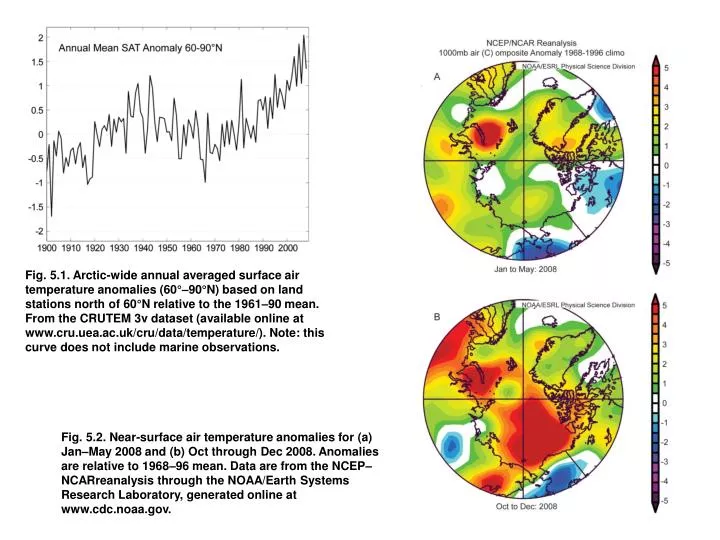
1. Fig. 5.1. Arctic-wide annual averaged surface air temperature anomalies (60°–90°N) based on land stations north of 60°N relative to the 1961–90 mean. From the CRUTEM 3v dataset (available online at www.cru.uea.ac.uk/cru/data/temperature/). Note: this curve does not include marine observations. Fig. 5.2. Near-surface air temperature anomalies for (a) Jan–May 2008 and (b) Oct through Dec 2008. Anomalies are relative to 1968–96 mean. Data are from the NCEP–NCARreanalysis through the NOAA/Earth Systems Research Laboratory, generated online at www.cdc.noaa.gov.

2. Fig. 5.3. An example of a positive AW pattern of SLP anomalies from Mar 2008. Purple/blue regions have relative low SLP and orange regions have high SLP. Anomalous winds tend to blow parallel to the contour lines, creating a flow from north of eastern Siberia across the North Pole. The orientation of the pressure dipole can shift; other examples have the anomalous geostrophic wind flow coming from north of the Bering Strait or Alaska. Data are from the NCEP–NCAR reanalysis available online at www.cdc.noaa.gov. Fig. 5.4. Vertical cross section from 60° to 90°N along 180° longitude averaged for Oct–Dec 2003 through 2008 (years for which summertime sea-ice extent fell to extremely low values) for (a) air temperature and (b) geopotential height. Data are from the NCEP–NCARreanalysis available online at www.cdc.noaa.gov.

3. Fig. 5.5. Simulated circulation patterns of the upper-ocean wind-driven circulation in (left) winter and (right) summer in 2008. Both patterns are identified as anticyclonic (clockwise). The intensity of anticyclonic circulation in summer 2008 has reduced relative to 2007 (see Proshutinsky and Johnson 1997 for details). Fig. 5.6. Satellite-derived summer (JAS) SST anomalies (Reynolds et al. 2002) in (left) 2007 and (right) 2008, relative to the summer mean over 1982–2006. Also shown is the Sep mean ice edge (thick blue line).

4. Fig. 5.7. Temporal (°C) and spatial variability of the AWCT. Locations of sections are depicted by yellow thick lines. Mooring location north of Spitsbergen is shown by a red star. There is a decline of Atlantic water temperature at 260 m at mooring locations with a rate of 0.5°Cper year starting at the end of 2006. Some cooling in 2008 is also observed at the sections crossing the continental slope in the vicinity of Severnaya Zemlya and in the east Siberian Sea (Polyakov et al. 2009, manuscript submitted to Geophys. Res. Lett.).

5. Fig. 5.8. (left) Summer heat (1 × 1010 J m−2) and (right) freshwater (m) content. Panels 1 and 3 show heat and freshwater content in the Arctic Ocean based on 1970s climatology (Arctic Climatology Project 1997, 1998). Panels 2 and 4 show heat and freshwater content in the Beaufort Gyre in 2008 based on hydrographic survey (black dots depict locations of hydrographic stations). For reference, this region is outlined in black in panels 1 and 3. The heat content is calculated relatively to water temperature freezing point in the upper 1000-m ocean layer. The freshwater content is calculated relative to a reference salinity of 34.8. Fig. 5.9. The 5-yr running mean time series: annual mean sea level at nine tide gauge stations located along the Kara, Laptev, east Siberian, and Chukchi Seas’ coastlines (black line). The red line is the anomalies of the annual mean AO Index multiplied by 3. The dark blue line is the sea surface atmospheric pressure at the North Pole (from NCAR–NCEP reanalysis data) multiplied by −1. Light blue line depicts annual sea level variability.

6. Fig. 5.10. Sea-ice extent in (left) Mar 2008 and (right) Sep 2008, illustrating the respective winter maximum and summer minimum extents. The magenta line indicates the median maximum and minimum extent of the ice cover, for the period 1979–2000. A—east Siberian Sea, B—Sea of Ohkotsh, C—Bering Sea, D—Beaufort Sea, and E—Barent’s Sea. (Figures from the NSIDCIndex: nsidc.org/data/seaice_index.) Fig. 5.11. Time series of the percent difference in ice extent in Mar (the month of ice-extent maximum) and Sep (the month of ice-extent minimum) from the mean values for the period 1979–2000. Based on a least-squares linear regression, the rate of decrease for the Mar and Sep ice extents was −2.8% and −11.1% per decade, respectively.

7. Fig. 5.12. Maps of age of Arctic sea ice for (left) 2007 and (right) 2008 in (top) Mar and (bottom) Sep. (top) Derived from QuikSCAT data (Nghiem et al. 2007). (bottom) Courtesy of C. Fowler, J. Maslanik, and S. Drobot, NSIDC, and are derived from a combination of AVHRR and SSM/I satellite observations and results from drifting ice buoys.

8. Fig. 5.13. (top, blue bars) Percentage change in sea-ice area in late spring (when the long-term mean 50% concentration is reached) during 1982–2007 along the 50-km-seaward coastal margin in each of the major seas of the Arctic using 25-km-resolution SSMIpassive microwave Bootstrap sea-ice concentration data (Comiso and Nishio 2008). (top, red bars) Percentage change in the summer land-surface temperature along the 50-km-landward coastal margin as measured by the SWI[sum of the monthly mean temperatures above freezing (°Cmo)] based on AVHRRsurface-temperature data (Comiso 2003). (bottom, green bars) Percentage change in greenness for the full tundra area south of 72°N as measured by the TI-NDVIbased on biweekly GIMMS NDVI(Tucker et al. 2001). Asterisks denote significant trends at p < 0.05. Based on Bhatt et al. (2008).

9. Fig. 5.14. (top left) Location of the long-term MIREKO and the Earth Cryosphere Institute permafrost observatories in northern Russia. (bottom left) Changes in permafrost temperatures at 15-m depth during the last 20 to 25 years at selected stations in the Vorkuta region (updated from Oberman 2008). (top right) Changes in permafrost temperatures at 10-m depth during the last 35 yr at selected stations in the Urengoy and Nadym (bottom right) regions (updated from Romanovsky et al. 2008).

10. Fig. 5.15. Total annual river discharge to the Arctic Ocean from the six largest rivers in the Eurasian Arctic for the observational period 1936–2007 (updated from Peterson et al. 2002) (red line) and from the five large North American pan-Arctic rivers over 1973–2006 (blue line). The least-squares linear trend lines are shown as dashed lines. Provisional estimates of annual discharge for the six major Eurasian Arctic rivers, based on near-real-time data from http://RIMS.unh.edu, are shown as red diamonds.

11. Fig. 5.16. (a) SCD anomalies (with respect to 1988–2007) for the 2007/08 snow year and (b) Arctic seasonal SCD anomaly time series (with respect to 1988–2007) from the NOAA record for the first (fall) and second (spring) halves of the snow season. Solid lines denote 5-yr moving average. (c) Maximum seasonal snow depth anomaly for 2007/08 (with respect to 1998/99–2007/08) from the CMCsnow depth analysis. (d) Terrestrial snowmelt onset anomalies (with respect to 2000–08) from QuikSCAT data derived using the algorithm of Wang et al. (2008a). The standardized anomaly scales the date of onset of snowmelt based on the average and the magnitude of the interannual variability in the date at each location. A negative anomaly (shown in red-yellow) indicates earlier onset of snowmelt in the spring.

12. Fig. 5.17. 2008 (a) winter and (b) summer near-surface (2 m) air temperature anomalies with respect to the 1971–2000 base period, simulated by Polar MM5 after Box et al. (2006).

13. Fig. 5.18. 2008 Greenland ice sheet surface melt duration anomalies relative to the 1989–2008 base period based on (a) SSM/Iand (b) QuikSCAT (2000–08 base period), after Bhattacharya et al. (2009, submitted to Geophys. Res. Lett.).

14. Fig. 5.20. 2008 surface mass balance anomalies with respect to the 1971–2000 base period, simulated by Polar MM5 after Box et al. (2006). Fig. 5.19. Surface albedo anomaly Jun–Jul 2008 relative to a Jun–Jul 2000–08 base period.