Download
1 / 45
450 likes | 574 Vues
Intensity Discrimination. Intensity discrimination is the process of distinguishing one stimulus intensity from another. Two types: Difference thresholds – the two stimuli are physically separate Increment thresholds – the two stimuli are immediately adjacent or superimposed. Fig. 1.1.

E N D
Intensity Discrimination Intensity discrimination is the process of distinguishing one stimulus intensity from another
Two types: Difference thresholds – the two stimuli are physically separate Increment thresholds – the two stimuli are immediately adjacent or superimposed
Fig. 1.1 Increment threshold stimuli (edges of stimuli touch each other) Difference threshold (separated stimuli)
Theory and Practice Theory:
Fig. 2.7 From Dr. Kraft’s course – Hecht, Shlaer & Pirenne Photon emission follows a Poisson distribution To distinguish a flash with a mean of 8 from a flash with a mean of 9 quanta is impossible! The distributions overlap almost completely
Mean of 8, vs. mean of 9 If present the flash with a mean of 8 photons many times and a flash with a mean of 9 photons presented many times, there will be many times that the 9 photon flash will have more photons than the 8 photon flash
In a Poisson distribution, the variance is equal to the mean. The standard deviation (SD) is the square root of the mean. In a two-alternative forced-choice task, to reach threshold (75% correct), LT must differ from L by 0.95 SD. (e.g., L = 0.95 SD)
Moreover, as L increases, the minimum threshold L also increases with the because the variance in a Poisson distribution equals the mean, so the SD changes with the square root of the mean
Theory and Practice In practice: at low background intensities, human observers behave as an ideal detector (follow the deVries-Rose Law)
You always can determine the Weber fraction, even when Weber’s Law does not hold
Fig. 3.2 Weber’s Law does NOT hold (L/ L rises as L decreases) Weber’s Law holds
Both the deVries-Rose and Weber’s laws fail to account for thresholds at high light intensities Fig. 3.3 The increment threshold data of a rod monochromat (circles) plotted along with the theoretical lower limit (deVries-Rose, dotted line) and the predictions of Weber’s 2 Law (solid line). Luminance values are in cd/m . (Redrawn from Hess et al. (1990)
More practical issues: How changes in other stimulus dimensions affect the Weber fraction
#1 Stimulus size: the Weber fraction is lower (smaller) for larger test stimuli Fig. 3.4
More practical issues: Is a target visible under certain conditions? D Log Weber Fraction, L/L 2 This is the target’s Weber fraction. It is NOT a threshold Test Field Diameter 4' 1 121' 0 Is a spot with a particular luminance, relative to background, visible? It depends on its size. -1 -2 If the target is 121’, it is visible If 4’, it is not visible -3 -7 -6 -5 -4 -3 -2 -1 0 1 2 3 2 Log Background Intensity, L (cd/m )
Need to distinguish between the Weber fraction of a target vs. the threshold of a viewer. For a subject or patient viewing a target, if the subject’s Weber fraction is below a line, then the subject’s threshold is better (smaller). If the Weber fraction of a target is below the line, the target is NOT visible to someone whose threshold is on the line.
The smaller the threshold L, the smaller is the value of the Weber fraction for a given background L, (only the numerator changes) and the more sensitive the visual system is to differences in light intensity.
The “dinner plate” example: Plate with luminance of 0.0102 footlamberts. Background is 0.01 footlamberts L is thus 0.0102– 0.01 = 0.0002. L/L = 0.0002/0.01 = 0.02 (plate is 2% more intense) From Figure 3-4, can learn that this is not visible.
More practical issues: Is a target visible under certain conditions? D Log Weber Fraction, L/L 2 Test Field Diameter 4' 1 Is a spot with a particular luminance, relative to background, visible? It depends on its size. 121' 0 Threshold Weber fraction for 121’ objects -1 -2 Plate’s Weber fraction -3 -7 -6 -5 -4 -3 -2 -1 0 1 2 3 2 Log Background Intensity, L (cd/m )
Continuing: How changes in other stimulus dimensions affect the Weber fraction #2 Short-duration flashes are harder to see (are less discriminable) than long-duration flashes That is, the threshold L increases as flash duration becomes shorter.
Continuing: How changes in other stimulus dimensions affect the Weber fraction #3 Threshold L varies with eccentricity from the fovea At low luminance levels, threshold is lowest (sensitivity is highest) about 15-20 degrees from fovea and the fovea is “blind” At high luminance levels, threshold is lowest at the fovea
Sensory Magnitude Scales Revisited Using the “just noticeable difference” (jnd) to create a scale for sensory magnitude vs. stimulus magnitude L + threshold L = LT LT is one jnd more intense than L. LT + threshold L = LT2 LT2 is one jnd more intense than LT And so on…
Sensory Magnitude 12 10 8 6 4 L 2 0 0 50 100 150 200 2 Stimulus Luminance, L (cd/m )
Sensory Magnitude 12 10 L + threshold L = LT LT is one “just noticeable difference” (jnd) more intense than L. 8 6 LT 4 L 2 0 0 50 100 150 200 2 Stimulus Luminance, L (cd/m )
Sensory Magnitude 12 LT + threshold L = LT2 LT2 is one jnd more intense than LT and 2 jnd’s larger than L 10 8 LT2 6 LT 4 L 2 0 0 50 100 150 200 2 Stimulus Luminance, L (cd/m )
Sensory Magnitude 12 LTn+1 10 LTn 8 When Weber’s Law holds, the threshold Ls keep getting larger, so 1 jnd is a larger increase in stimulus luminance LT2 6 LT 4 L 2 0 0 50 100 150 200 2 Stimulus Luminance, L (cd/m )
Fechner’s Law Sensory Magnitude 12 10 8 6 4 2 Fechner's Law: Log(L) 0 0 50 100 150 200 2 Stimulus Luminance, L (cd/m )
Comparing Fechner’s Law with Stevens’ Power Law Fig. 3.6 Stevens’ Power Law resembles Fechner’s Law when the exponent is <1