Tracking of Varying Mean Transit Time

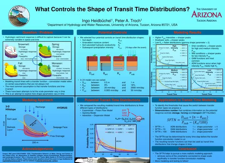
1. What Controls the Shape of Transit Time Distributions? Ingo Heidbüchel1, Peter A. Troch11Department of Hydrology and Water Resources, University of Arizona, Tucson, Arizona 85721, USA Question / Problem Potential Controls Tracking of Varying Mean Transit Time Modeling Results • Hydrologic catchment response is difficult to capture because it can be extremely variable in space and time • We selected four potential controls on transit time distribution shapes: • Soil depth Dsoil • Antecedent moisture content θant • Soil saturated hydraulic conductivity Ks • Subsequent precipitation intensity Psub (10 days after theevent) • In 24 model runs we varied: • Dsoil between 0.5 m and 1 m • θantbetween 9% and 18% • Ksbetween 20 mm/dayand 2000 mm/day • Psubbetween 0.005 mm/dayand 50 mm/day • Higher Psub intensities =sharper peaks • Shallower soils =sharper peaks • Low Ks=flatter distributions (gamma shape parameter > 2) 0.12 0.1 0.08 0.06 0.04 0.02 0 ADM 4.0 ADM 1.4 ADM 1.2 GAM 1.0 GAM 2.2 High IntensityPsub • Drier conditions = sharper peaks for high and medium intensity Psub • Wet conditions = sharper peaks for low intensity Psub • GAM functions are most common • ADM functions occur when high intensity Psub meets high Ks Shallow Dry HighKs Snowmelt: Storage increasing Hydrologic response fast Flowpaths slow / intermediate / fast Spring: Storage decreasing Hydrologic response intermediate Flowpaths slow / intermediate Deep Dry HighKs Probability Density Shallow Wet HighKs Overland Flow Deep Wet HighKs Interflow Deep Wet LowKs Base Flow 0 20 40 60 80 100 Fall: Storage decreasing Hydrologic response slow Flowpaths slow Monsoon: Storage constant / increasing Hydrologic response intermediate / fast Flowpaths intermediate / fast 0.06 0.05 0.04 0.03 0.02 0.01 0 ADM 1.4 GAM 0.95 GAM 1.0 GAM 2.3 GAM 2.4 Medium IntensityPsub GAM 0.8 GAM 0.95 ADM 6500 GAM 1.9 GAM 2.2 GAM 2.4 Low IntensityPsub Dsoil θant Ks Psub Shallow Wet HighKs Shallow Dry HighKs DeepWet HighKs Deep Dry HighKs Probability Density Shallow Wet LowKs Shallow/Deep Wet HighKs • Modeling transit times with a transfer function – convolution model relies on certain assumptions that are not always met • The most common assumption is that transfer functions are time-invariant • There have been attempts to let the scale parameter vary in time • This is an attempt to explore how shape parameters vary in time Deep Dry/Wet LowKs Shallow Wet LowKs Shallow Dry LowKs Deep Wet LowKs Shallow/Deep Dry HighKs 0 20 40 60 80 100 0 20 40 60 80 100 Transit Time Transit Time Application to Transit Time Modeling Modeling Approach Potential Transit Time Distributions • We compared the resulting modeled transit time distributions to three different types of distributions: • Exponential – Piston Flow Model EPF • Gamma Model GAM • Advection – Dispersion Model ADM • To identify the thresholds that cause the switch between transfer function types we propose a • Dimensionless number that combines information on the potential response controls storage, forcing and transport (SFT-Number): 3-D Hillslope Recharge HYDRUS Soil Layer 0.06 0.05 0.04 0.03 0.02 0.01 0 EPF 1.1 GAM 0.5 ADM 0.5 EPF 1.25 GAM 1 ADM 1 EPF 1.5 GAM 2 ADM 2 45 m 40 m • SFTN < 1: ADM distributions 1 < shape parameter < 4 • SFTN > 10: GAM distributions 1 < shape parameter < 2 • SFTN > 100: GAM distributions 2 < shape parameter • The SFTN can be determined for every time step before the transfer function-convolution model is run • The resulting transfer functions can then be used as transit time distributions that change shapes in time Bedrock Layer Seepage Face Probability Density Free Drainage MEAN 200 m Acknowledgements Conclusion δout(t) = ∫δin (t-τ) * Vin (t-τ) * TTDv(τ)dτ ∫Vout (t-τ) * HRFv(τ)dτ 0 20 40 60 80 100 • The SFTN helps to pursue a more realistic modeling approach • removes some of the uncertainty connected to shape-scale equifinality in transfer function-convolution modeling • More modeling and testing to follow! Time Project: NSF grant EAR-0724958 “CZO: Transformative Behavior of Water, Energy and Carbon in the Critical Zone: An Observatory to Quantify Linkages among Ecohydrology, Biogeochemistry, and Landscape Evolution” (PIs: J. Chorover and P.A. Troch). Many thanks to Ty Ferré for providing us with the Hydrus software. Please direct further questions about this poster to Ingo Heidbüchel at ingohei@hwr.arizona.edu or visit our website at www.hwr.arizona.edu/~surface.