Download
1 / 1
10 likes | 96 Vues
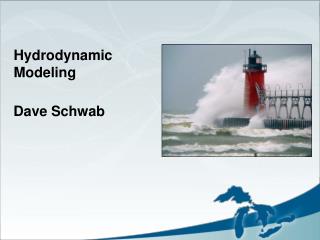
XRBs in 2d: Hydrodynamic Modeling of a 4 He Burst Prior to Peak Light Chris Malone 1 , A. S. Almgren 2 , J. B. Bell 2 , A. J. Nonaka 2 , M. Zingale 1 1 Dept. of Physics and Astronomy, SUNY Stony Brook, 2 CCSE / LBNL.

E N D
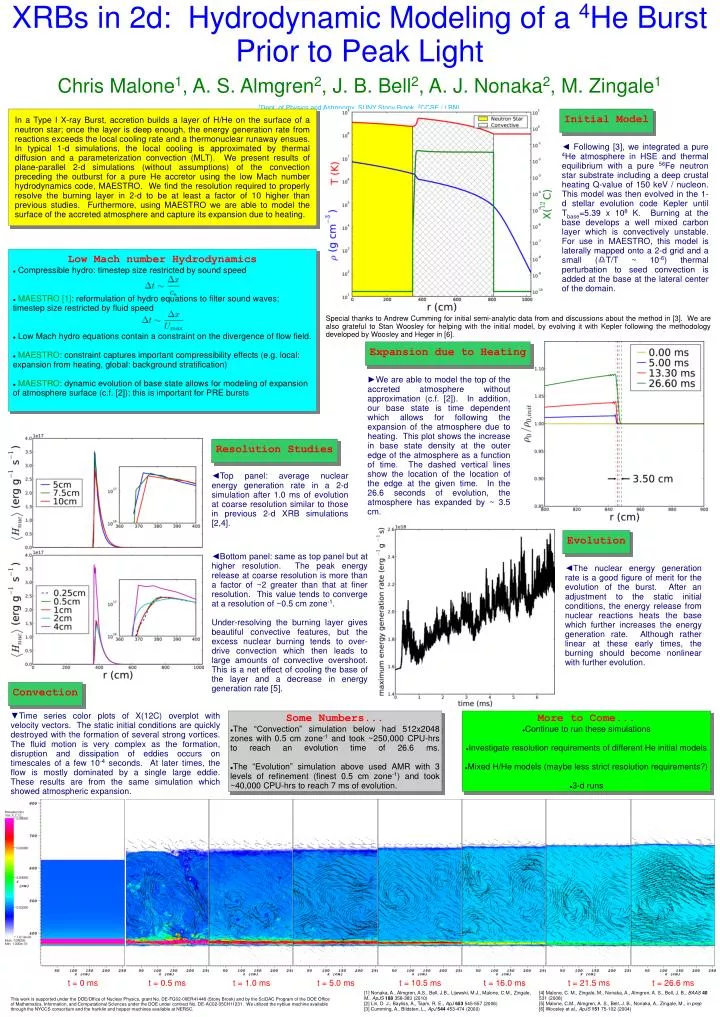
XRBs in 2d: Hydrodynamic Modeling of a 4He Burst Prior to Peak Light Chris Malone1, A. S. Almgren2, J. B. Bell2, A. J. Nonaka2, M. Zingale1 1Dept. of Physics and Astronomy, SUNY Stony Brook, 2CCSE / LBNL In a Type I X-ray Burst, accretion builds a layer of H/He on the surface of a neutron star; once the layer is deep enough, the energy generation rate from reactions exceeds the local cooling rate and a thermonuclear runaway ensues. In typical 1-d simulations, the local cooling is approximated by thermal diffusion and a parameterization convection (MLT). We present results of plane-parallel 2-d simulations (without assumptions) of the convection preceding the outburst for a pure He accretor using the low Mach number hydrodynamics code, MAESTRO. We find the resolution required to properly resolve the burning layer in 2-d to be at least a factor of 10 higher than previous studies. Furthermore, using MAESTRO we are able to model the surface of the accreted atmosphere and capture its expansion due to heating. Initial Model ◄ Following [3], we integrated a pure 4He atmosphere in HSE and thermal equilibrium with a pure 56Fe neutron star substrate including a deep crustal heating Q-value of 150 keV / nucleon. This model was then evolved in the 1-d stellar evolution code Kepler until Tbase=5.39 x 10⁸ K. Burning at the base develops a well mixed carbon layer which is convectively unstable. For use in MAESTRO, this model is laterally mapped onto a 2-d grid and a small (dT/T ~ 10-6) thermal perturbation to seed convection is added at the base at the lateral center of the domain. • Low Mach number Hydrodynamics • Compressible hydro: timestep size restricted by sound speed • MAESTRO [1]: reformulation of hydro equations to filter sound waves; timestep size restricted by fluid speed • Low Mach hydro equations contain a constraint on the divergence of flow field. • MAESTRO: constraint captures important compressibility effects (e.g. local: expansion from heating, global: background stratification) • MAESTRO: dynamic evolution of base state allows for modeling of expansion of atmosphere surface (c.f. [2]); this is important for PRE bursts Special thanks to Andrew Cumming for initial semi-analytic data from and discussions about the method in [3]. We are also grateful to Stan Woosley for helping with the initial model, by evolving it with Kepler following the methodology developed by Woosley and Heger in [6]. Expansion due to Heating ►We are able to model the top of the accreted atmosphere without approximation (c.f. [2]). In addition, our base state is time dependent which allows for following the expansion of the atmosphere due to heating. This plot shows the increase in base state density at the outer edge of the atmosphere as a function of time. The dashed vertical lines show the location of the location of the edge at the given time. In the 26.6 seconds of evolution, the atmosphere has expanded by ~ 3.5 cm. Resolution Studies ◄Top panel: average nuclear energy generation rate in a 2-d simulation after 1.0 ms of evolution at coarse resolution similar to those in previous 2-d XRB simulations [2,4]. Evolution ◄Bottom panel: same as top panel but at higher resolution. The peak energy release at coarse resolution is more than a factor of ~2 greater than that at finer resolution. This value tends to converge at a resolution of ~0.5 cm zone-1. Under-resolving the burning layer gives beautiful convective features, but the excess nuclear burning tends to over-drive convection which then leads to large amounts of convective overshoot. This is a net effect of cooling the base of the layer and a decrease in energy generation rate [5]. ◄The nuclear energy generation rate is a good figure of merit for the evolution of the burst. After an adjustment to the static initial conditions, the energy release from nuclear reactions heats the base which further increases the energy generation rate. Although rather linear at these early times, the burning should become nonlinear with further evolution. Convection ▼Time series color plots of X(12C) overplot with velocity vectors. The static initial conditions are quickly destroyed with the formation of several strong vortices. The fluid motion is very complex as the formation, disruption and dissipation of eddies occurs on timescales of a few 10-4 seconds. At later times, the flow is mostly dominated by a single large eddie. These results are from the same simulation which showed atmospheric expansion. • Some Numbers... • The “Convection” simulation below had 512x2048 zones with 0.5 cm zone-1 and took ~250,000 CPU-hrs to reach an evolution time of 26.6 ms. • The “Evolution” simulation above used AMR with 3 levels of refinement (finest 0.5 cm zone-1) and took ~40,000 CPU-hrs to reach 7 ms of evolution. • More to Come... • Continue to run these simulations • Investigate resolution requirements of different He initial models • Mixed H/He models (maybe less strict resolution requirements?) • 3-d runs t = 0 ms t = 0.5 ms t = 1.0 ms t = 5.0 ms t = 10.5 ms t = 16.0 ms t = 21.5 ms t = 26.6 ms [1] Nonaka, A., Almgren, A.S., Bell, J.B., Lijewski, M.J., Malone, C.M., Zingale, M., ApJS188 358-383 (2010) [2] Lin, D. J., Bayliss, A., Taam, R. E., ApJ653 545-557 (2006) [3] Cumming, A., Bildsten, L., ApJ544 453-474 (2000) [4] Malone, C. M., Zingale, M., Nonaka, A., Almgren, A. S., Bell, J. B., BAAS40 531 (2008) [5] Malone, C.M., Almgren, A. S., Bell, J. B., Nonaka, A., Zingale, M., in prep [6] Woosley et al., ApJS151 75-102 (2004) This work is supported under the DOE/Office of Nuclear Physics, grant No. DE-FG02-06ER41448 (Stony Brook) and by the SciDAC Program of the DOE Office of Mathematics, Information, and Computational Sciences under the DOE under contract No. DE-AC02-05CH11231. We utilized the nyblue machine available through the NYCCS consortium and the franklin and hopper machines available at NERSC.