Download
1 / 1
10 likes | 99 Vues
Simulation of Patterned Plant Growth in Extreme Environments. CSUSB Institute For Applied Supercomputing. 0. 1. 1. Time = t 0. 1. 0. S. 0. 0. 0. Time = t 1. 1. J. Curnutt, E. Gomez, K. Schubert. Introduction. Cellular Automaton.

E N D
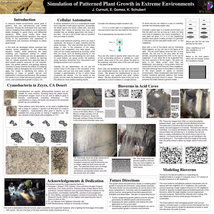
Simulation of Patterned Plant Growth in Extreme Environments CSUSB Institute For Applied Supercomputing 0 1 1 Time = t0 1 0 S 0 0 0 Time = t1 1 J. Curnutt, E. Gomez, K. Schubert Introduction Cellular Automaton To show how this can relate to a case of crowding, consider the following simple rules. Consider a plant type in a hostile environment, so that the plant can live as long as it does not have more than 6 neighbors (too much competition). A new plant will grow if 2 or 3 of the neighboring squares have plants (it takes at least 2 to generate a new plant, but the new plant needs room- i.e. few neighbors). Start with a row of five plants and an interesting thing happens, as you can see in the figure at the right. The ten small figures show the first 10 time periods, the last one is the area after 40 time periods, assuming beyond this limit no life can be supported. If you allow life to be supported then the lines continue to fill the region. No plant can grow in the “dead zones” once they are established, and placing a living plants there will cause them to die (it will have too many neighbors). This self-enforcing nature of the pattern is the basis of the maze growth of plants in extreme environments. More complicated rules that fit more realistic situations generate patterns that imitate the striking structures found in nature. This poster presents first steps toward a general model. In resource limited environments, plants grow in patterns that are self-enforcing and exhibit hysteresis. Among the techniques that have been used to modeling these patterns are evolutionarily stable strategies in game theory and differential equations. While good results have been generated using differential equations, they require tuning of the parameters and experience in mathematical and numerical techniques to obtain good results. In this work we developed cellular automata that achieve similar predictions to the differential equation models, while preserving the rapid modeling and hypothesis testing of cellular automata. Similar models can also be applicable to group animal behavior. Our method for deriving rules for cellular automata from observed data in plant growth patterns accounts for soil nutrients, water, root growth patterns, and geology allowing scientists to easily examine the effects of modifying conditions without damaging the environment. We apply this model to identifying the factors of patterning in areas of growth, die-out, and stabilization in extreme environments. We compare the results of our model with bioverm growth in acid caves, and cyanobacteria growth in Zzyzx, CA. A cellular automaton (CA) is a computational model that is discrete in both space and time. Essentially we divide space into boxes called cells, and only calculate their values at discrete time (you could consider this as dividing space-time into boxes if you like). CA use a set of fixed rules to transition from one state to another. A state could represent anything, and in our case it represents the amount of water, nutrients and the plants biomass. The rules describe how the plant grows or dies in the presence of the water, nutrients and competition from other plants. CA rules are not usually expressed as formulas, rather they are visual, such as drawing pictures of the neighboring cells and then labeling the next state. To avoid tedium, we group similar cell patterns using heuristics discerned from discussions with biologists and born out in practice. Typically CA are deterministic, do not use the current value of the state in the calculation of the next state, and use only one state variable. We consider a generalization of this in which these constraints are relaxed. For the results on this poster, we only relax the determinism constraint, as this allows for more realistic looking results. Consider the following simple transition rule. If 3 or 4 of the cells in a neighborhood of ±1 row and column then the next state for the cell is 1. This is illustrated by the transition of cell S: Thus we only need to specify what value the sum of the surrounding biomass is needed for plant growth, what value of the sum allows the plant to be sustained, and what value of the sum will result in the plant’s death. Such rules are deceptively simple, but can lead to very complicated results, as the rest of the poster shows. We allowed the neighborhood to vary to simulate plant root systems and other nutrient effects. We also allowed the value of the sum to be specified as a list of numbers or a single interval. Above are the first ten time periods for the rules: Grow: neighbors=2 or 3 Die: neighbors > 6 Same: else Below is the final patern, which will not change unless the conditions change. Cyanobacteria in Zzyzx, CA Desert Bioverms in Acid Caves Cyanobacteria are aquatic, photosynthetic bacteria and are notable for many reasons, including being the oldest fossils, atmospheric oxygen, much of our oil, and an ability to grow in extreme environments (including Antarctica). The cyanobacteria in Zzyzx are fossils, but preserve the structured growth we are considering. These patterns were fairly dense, so we used a neighborhood with a range of 1 square (1 square in all directions for a total of 8 neighbors). Cyanobacteria often grow in blooms, so we modeled this using growth on having 3 neighbors only. We also allowed random death with probability of 10%. PB- From Cueva de Luna Azufre (Cave of the Sulfur Moon), in Tabasco, Mexico (image courtesy of K.W. Stafford), this picture shows the thorough coating of these formations in this small and extremely nasty cave. PB- These two images from Villa Luz show boundaries between black, ragu, and light colored (lithified) bioverms. The white part is bioverms that are lithified, mainly with calcite, but some gypsum is involved. The black and red are unlithified. It is hard to tell whether the white is older and the red and black has formed over it, or whether the red and black is simply unlithified but the whole thing is part of one deposit. It is hard to tell even when you are standing in the cave looking at it. The height of the first image of the whole wall, the white streak is about my height, about 5 and a half feet. T=100 T=30 T=40 PB- And finally, there are large exposures of limestone where the conditions have changed (I presume) and the bioverms are no longer viable but faint traces are still seen. The attached shows such an image. They are shriveled and dried and the connections are typically broken and only the central nexii are visible. PB- This image shows the bioverm patterns and how they can come together so thickly that it becomes a solid carpet. Modeling Bioverms The key to the bioverm patterns is expanding the neighborhoods to a range of 3 squares, thus a 7x7 section of the grid (maximum of 48 neighbors). The more freeform and globular patterns had growth only for spaces with few neighbors (8-11 neighbors), but continued survival requiring a larger support structure (21-40 neighbors). Growth in sparsely occupied areas promoted expansion of the bioverms, while the large neighbor survival requirement ensured clumping. Note that the intervals don’t overlap, this was deliberate to remove small groups that were not sustainable. The linear patterns had overlapping growth and survival regions, and were given a nutrient source that flowed from the roof. This was done to model the dissolved minerals in water that drip down the walls of caves. Future Directions Acknowledgements & Dedication Penelope Boston at work This poster shows the preliminary results of modeling plant growth in extreme environments, using cellular automata. The early results are very promising, as can be seen in the photo comparisions. Currently rules are established in an ad-hoc manner, using general heuristics gleaned from biologists and observation. We plan on expanding this by: • The Authors would like to give special thanks to: • Penelope J. Boston, PhD, Director, Cave and Karst Studies Program and Assoc. Prof. Earth and Env. Sciences Dept. at New Mexico Tech and Assoc. Director National Cave and Karst Research Institute for the cave photos, commentary marked PB-, and lots of encouragement. • Dr. Chris McKay, principal investigator, extreme environments, Ames Research Center, NASA, for the impetus and organizing two trips to Zzyzx to work on this. • Dr. Jim Nienow, from Valdosta University, GA. • NSF BioAstronomy Institute at University of Hawaii. • Further categorizing growth patterns and the relevant parameters for different plants and environments. • Expanding the state variables and making the rules dependent on the current state. • Developing a graphical interface biologists can use to examine plant growth in extreme environments. This work is dedicated to Norval Curnutt, Jane’s wonderful and supportive husband, who is fighting the final stage of his battle with cancer. Norval is the best of the best and will be sorely missed by all of us.