Download
1 / 36
420 likes | 713 Vues
Magnetic Fields. Madhawa Hettiarachchi, PhD LPPD Director Prof. Andreas A. Linninger 06/23/2010. Out Line. Motivation History Laws Magnetic dipoles Ferromagnetic materials Maxwell equations Electromagnetic waves Magnetic Particle Motion. What do we mean by Magnetic Field ?.

E N D
Magnetic Fields Madhawa Hettiarachchi, PhD LPPD Director Prof. Andreas A. Linninger 06/23/2010
Out Line • Motivation • History • Laws • Magnetic dipoles • Ferromagnetic materials • Maxwell equations • Electromagnetic waves • Magnetic Particle Motion
What do we mean by Magnetic Field? • A Magnetic field is produced by • whenever there is electrical charge in motion • a permanent magnet (orbital motions and spins of electrons) • Magnetic fields exerts force on both moving electrical charges and permanent magnets.
Motivation Many useful and important technologies are underpinned by our knowledge of magnetic phenomena: • Data Storage/read/write • Entertainment: home theatre • Medical: Magnetic Resonance Imaging (MRI) Drug Transport • Transport: electric trains, Maglev trains….
Brief History • Danish physicist Hans Oersted found in 1819 that a current flowing in a wire deflected a compass needle.
Brief History Cont. • Andre Ampere (1775-1836) repeated Oersted’s experiments and formulated the right hand rule in the early 1820s. • Ampere’s essential contribution was to show that electricity and • magnetism were part of the same phenomenon(prior to 1820 they had been seen as separate branches of science.)
Brief History Contd. In 1831 English physicist Michael Faraday discovered electromagnetic induction, The magnetic flux Φ is the normal component of B integrated over surface S: The magnetic flux Φ has units Webers. (1Tesla=1Weber/m2) This leads to the invention of motor.
Electric and Magnetic forces on a moving charge: Lorentz force Magnetic force. This is an empirical fact. This force is perpendicular to the velocity, v, of the charge. The direction of the charge’s velocity is changed; the magnitude of the velocity is not changed. Electric force is straight forward. It is in the same direction as the electric field.
Force on a current-carrying wire An electric current is a movement of charge along a wire. Current is in amperes (A) or coulombs per second (Cs-1)
Biot-Savart law Who were they? Biot: French physicist (1774-1862) who worked on optics and took a lot of scientific apparatus up in a hot air balloon with fellow physicist Gay-Lussac... Savart: French professor (1791-1841) at the College de France. Collaborated with Biot. What does the law do for us? Tells us how to calculate the magnetic induction B due to steady currents. We now use the Biot-Savart law to deal with problems in magnetostatics: this is the situation of steady currents leading to constant magnetic fields.
Biot-Savart law contd.. Consider a current carrying wire in an arbitrary geometry: The Biot-Savart law gives us: dl is an integration element of length along the current path. r is a position vector pointing from the element of circuit dl towards the field point at which we want to know B. The magnetic induction B is measured in SI units teslas (T). The constant μ0 =4π x 10−7 tesla metre/ampere is called the permeability of free space.
Biot-Savart law contd. How big is 1 tesla? B is often given in the non-SI unit of gauss: 1T = 104 gauss. Earth’s magnetic field is ~ 1/2 gauss. So 1T is ~ 20,000 x Earth’s field. For comparison, A small bar magnet will produce B ~10-2 T MRI body scanner magnet B ~2T Big electromagnet B ~1.5 T Strong lab magnet B ~10 T Colour TV B ~ 10-6 T Surface of a neutron star is thought to be B ~108 T. Magnetometer It will show polarity and magnitude of the field.
Ampere’s law -Another way to calculate B field. Who was Amperè? André Marie Amperè (1775-1836) grew up in the S. of France but still managed to submit his first mathematical paper to the Academy de Lyon at age 13! The family was beset by tragedy: Amperè’s sister died when he was only 17. Amperè’s father was sent to the guillotine for upsetting the authorities in Paris. Ampere married Julie who is recorded to have said of him on their first meeting, “He has no manners; he is awkward, shy and presents himself badly” . Despite all the setbacks Ampere made fundamental contributions to the establishment of EM theory in the 19th C and he is remembered in the name of the unit for electric current. What does Amperè’s law do? Amperè’s law gives us an elegant method for calculating the magnetic field – but only in cases where the symmetry of the problem permits (otherwise we must use the Biot-Savart Law). Amperè’s law is to magnetics as Gauss’ law is to electrostatics.
Ampere’s law contd. If we have a volume current density, J, enclosed (not just a wire carrying current I) we can write, Relates the integrated magnetic field around a closed loop to the electric current passing through the loop
Gauss’s law Integral form The net magnetic flux out through any closed surface is zero Differential form This tells us there are no magnetic ‘monopoles’ (perhaps we might say, no ‘magnetic charges’) in nature.
Magnetic Dipoles Size of the dipole a <<< Z Expressions for magnetic and electric dipole fields in the free space: How field changes within a materials?
Magnetic Materials So far we have limited our discussion to the effects currents in conductors that generate fields in free space (where the permeability is μ0=4πx10-7). But the permeability is not (generally) μ0 in materials. In matter, the electrons in motion in atomic orbitals may be viewed as an assembly of microscopic current loops or magnetic dipoles. If we put matter in a magnetic field B, these magnetic dipoles tend to align with respect to B. In diamagnetic and paramagnetic materials the alignment is small. In ferromagnetics, alignment is almost complete over regions called domains. The macroscopic, measurable property of a material due to its internal, microscopic dipole arrangement is called the magnetization of the material. Magnetization has the vector symbol M and measures the dipole moment of the material.
Magnetic Materials contd. Magnetization M is the magnetic dipole moment per unit volume. M is measured in units amperes per metre, Am-1. If each atom has magnetic dipole moment m and there are N atoms per unit volume, then magnetization M = Nm. Ferromagnetism is a strong magnetic effect: permanent magnets exhibit ferromagnetism – they can drive loudspeakers, start car engines, etc. Effects of paramagnetism and diamagnetism are usually too weak to be obvious (i.e. not easily observable, unless the B is very intense). In a non-uniform B paramagnetic objects are attracted into the field, diamagnetic objects are repelled out.
H- magnetic field intensity μ0- permeability of free space - magnetic susceptibility Magnetic Materials contd. Field inside a material :
Magnetic Materials contd. An iron core has the effect of multiplying greatly the magnetic field of a solenoid compared to the air core solenoid on the left. Relative permeability Why iron creates strong B field?
Ferromagnetic Materials contd. This strong (large) spin alignment leads to huge permeabilities: Material Relative Permeability μr Nickel 250 Cobalt 600 Iron (pure) 4,000 Mumetal(alloy) 100,000 Compare to paramagnetic metal: Aluminium ≈ 1
Maxwell’s equations in integral form Maxwell’s equations in integral form perhaps give us a greater physical insight: Electric flux through any closed surface equal to the electric charge within the surface. The total magnetic flux through any Gaussian surface is zero Electric field can be created by changing magnetic field. Magnetic field can be generated by electrical current or/and by changing electric fields
Maxwell’s Equations in differential form We can now write the complete set of Maxwell equations, including the correction term:
Maxwell’s Equations contd. Maxwell’s Equations tell us how CHARGES produce FIELDS and the force equation (electric + magnetic force acting on a moving charge) F=q(E+vxB) tells us how FIELDS affect CHARGES which together with the equation of continuity ∇.J = − ∂ρ/∂t provide all the mathematical apparatus needed to describe electromagnetism – that is to solve all problems in classical electromagnetism on the macroscopic scale.
Visualization of Maxwell’s equations Electric flux through any closed surface equal to the electric charge within the surface. Lines of E begin on positive charges. E lines exit enclosing volume τ through surface S. Gauss’ law says the total flux of E leaving enclosed volume τ is equal to the total charge enclosed by surface S divided by ε0.
The total magnetic flux through any Gaussian surface is zero Lines of magnetic induction B pass through the closed surface S. The net outward flux (divB) through the surface is zero. Gauss divergence theorem states, for any ‘well-behaved’ vector field A,
Electric field can be created by changing magnetic field. The emf induced in the loop L defined on surface S is equal to the rate of change of the magnetic flux through the surface enclosed by L.
Magnetic field can be generated by electrical current or/and by changing electric fields The arrows on the diagram above give the direction of the free current J. If D is downward and increasing or upward and decreasing the displacement current JD= ∂ D/∂t is also in the downward direction
Electromagnetic Waves Classical wave equation Maxwell’s equations give propagating EM waves If we take the two Maxwell eqns. (in differential form) and take the curl of these two in a region of space with • no charge • no current Take curl of (iii):
Electromagnetic Waves contd.. These equations describe electromagnetic waves EM propagating at velocity c (velocity of light). Electromagnetic waves transmit information and power. James Clerk Maxwell (1831-1879), Scottish mathematician and physicist in “A Treatise on Electricity and Magnetism” (1873) first showed that the Maxwell’s equations implicitly require the existence of EM waves traveling at the speed of light.
u r Fd Fm Φ Magnetic Dipole Magnetic Particle Motion in a Gradient Field Magnetic field inside the fluid due to the line pole Force on the particle Drag force on the flow Rm-particle radius Vm-particle volume mm- mass of the particle Force balance on the particle
Questions Thank you