Download
1 / 32
491 likes | 1.17k Vues
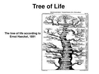
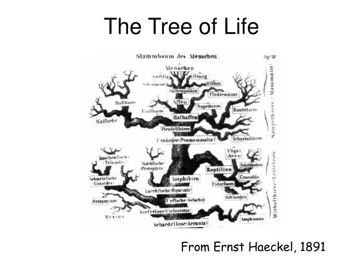
The Tree of Life. From Ernst Haeckel, 1891. But, is there only one “Tree of Life?”. There are many theories of evolution Basic idea: Speciation is caused by physical separation into groups where different genetic variants become dominant

E N D
The Tree of Life From Ernst Haeckel, 1891
But, is there only one “Tree of Life?” • There are many theories of evolution • Basic idea: • Speciation is caused by physical separation into groups where different genetic variants become dominant • Basic Tennant: Any two species share a common ancestor some time in the distant past
We are generally considering a “Gene Tree” as opposed to a “Species Tree.” • Divergence within a gene generally happens before splitting into species occurs. • In order to get a picture of evolution involving species, there is a need to look at collections of genes as opposed to individual genes.
Classical phylogenetic analysis: morphological features • number of legs, lengths of legs, etc. • Modern biological methods allow for the use of molecular features • Gene sequences • Protein sequences • Analysis based on homologous sequences (e.g., globins) in different species
Use of Molecular Data • Provides an objective criteria for constructing phylogenetic trees • Basic data includes • Gene sequences • Protein sequences • Analysis based on homologous sequences in different species
However, gene/protein sequence can be homologous for different reasons: Orthologs -- sequences diverged after a speciation event Paralogs -- sequences diverged after a duplication event Xenologs -- sequences diverged after a horizontal transfer (e.g., by virus)
1 2 1 3 2 3 1 6 Two main kinds of information are contained in trees: The tree topology The tree metric The form or shape of the tree distance or branch length
NO! YES! Cycle Family trees can look like this These two trees are topologically equivalent. The one on the right is more common in biology texts.
II I III I IV II III V V IV Trees can be unrooted or rooted
If there are n leaf nodes or taxa, how many different trees are possible? NR = Number of Possible Rooted Trees = NU = Number of Possible Unrooted Trees = The numerator contains the computationally insidious factorial function. Well, so does the denominator, but it is for a much smaller number.
B A C A C B D D Three Leaf Nodes B A C Only one unrooted tree is possible Four Leaf Nodes C B A D Three different unrooted trees are possible
A Table Showing the Growth of n! What do you notice in this table? Why is this true?
To Further Make the Point If we are creating a tree with 15 different taxa, there are 213,458,046,767,875 possible rooted trees. Assuming a computer can create a tree in 10-9 seconds, it would take 2.47 days of computation time to create them. If 20 species, 8,200,794,532,637,891,559,337 possible trees and the same computer would take 259,867 years to generate this many trees!
If we assume the Molecular Clock is working, then the distance from the root to each leaf is the same. The above tree does not assume a Molecular Clock!
Distance data can be generated from character data: Jukes-Cantor where p = percent of mismatches Kimura where P = percent transitions Q = percent transversions
Next we create a matrix of these distances For Example:
Simple Distance-Based MethodUnweighted-pair-group method with arithmetic mean Input: distance matrix between species Outline: • Cluster species together • Initially clusters are singletons • At each iteration combine two “closest” clusters to get a new one
UPGMA Clustering • Let Ci and Cj be clusters, define distance between them to be • When combining two clusters, Ci and Cj, to form a new cluster Ck, then
0.5 0.5 B D Begin with the following distance matrix Closest Pair is {B, D} so cluster them, C1 = {B, D} d(C1,A) = 1/2 (4 + 4) = 4 d(C1,C) = 1/2 (4 + 4) = 4 d(C1,E) = 1/2 (4 + 4) = 4 Tree at end of Stage 1
0.5 0.5 B D 1 1 A C Create a new matrix that includes C1 Closest are A and C, so C2 = {A, C} d(C1, C2) = 1/2 (4 + 4) = 4 d(C2, E) = 1/2 (3 + 3) = 3 Tree at end of Stage 2
0.5 0.5 1.5 0.5 0.5 1 1 1.5 B D A C E Once again we revise the distance matrix: We create group C3 = {C2, E} ={{A, C}, E} d(C1, C3) = 1/6 ( d(B,A) + d(B,C) + d(B,E) + d(D,A) + d(D,C) + d(D,E)) = 1/6(4+4+4+4+4+4)=4 NOTE: This tree satisfies the Molecular Clock Assumption. This is a basic property of UPGMA produced trees. Completed Tree
The Fitch-Margoliash(FM) Algorithm • A weaker requirement is additivity • In “real” tree, distances between species are the sum of distances between intermediate nodes k c b j a i
Consequences of Additivity • Suppose input distances are additive • For any three leaves • Thus k c b j a m i
A x z C y B Applying this idea to three taxa, A, B, and C: Using the fact that: x + y = d(A,B) x+ z = d(A,C) y + z = d(B,C) and a little high school algebra, we have x = 1/2 (d(A,B) + d(A,C) – d(B,C)) y = 1/2 (d(A,B) + d(B,C) – d(A,C)) z = 1/2 (d(A,C) + d(B,C) – d(A,B)
We will apply this criterion to the following data: We note that A and B are the closest, but to group them without the assumption of equal distance from a common ancestor, we temporarily group C-D-E and use the three taxa case: d(A,C-D-E) = 1/3(1.01+.75+1.03) = .93 d(B,C-D-E) = 1/3(1.00+.69+.90) = .863
From the formulas two slides previous we have: A .1885 .7415 C-D-E .1215 B Recall, the joining of C-D-E was only temporary so that we could get accurate distances for joining A and B Separating C, D, and E and combining A and B for the rest of the algorithm gives the table:
We now have the table: The closest distance is D,E. So we combine everything else into a single group A-B-C d(D,A-B-C) = 1/3(.75+.69+.61) = .683 d(E,A-B-C) = 1/3(1.03+.90+.42) = .783
This yeilds an intermediate tree of: D .135 .548 A-B-C .235 E We keep the edges joining D and E while discarding the grouping A-B-C. We now have four edges of our tree and two groupings. d(A-B,D-E) = 1/4 (.75+1.03+.69+90) = .8425 d(A-B,C) = .72 d(C,D-E) = 1/2 (.61+.42) = .515
We can now produce the table: Again applying the distance formulas we have the tree: C .33875 .6625 A-B .17625 D-E
0.33875 0.1885 0.135 a b 0.1215 0.235 C A D B E All that remains is to compute a and b The average of A and B from their common vertex is 0.155. For D and E the average distance is .185 So for the value of a we have .66625 – .155 = .51125 for the value of b we have .1765 – .185 = -.00875 The negative value for b is a cause for concern about the quality of our data. If we are confident of our data and since .00875 is close to 0, most researchers would assign a value of 0 to b.
One concern is that we have produced an unrooted tree for our five species is that we have an unrooted tree and no real clue on where to place the root. Sometimes physical evidence can help with the placement of a root for the tree; however, many times such evidence does not exist. A common heuristic practice is to include an extra taxon that is more distantly related to those under consideration than they are to each other. Such a taxon is called an outgroup. The biological asumption is that this group must have split from the others before they split from themselves.