Download
1 / 27
340 likes | 676 Vues
Genetic diversity and evolution. Content. Summary of previous class H.W equilibrium Effect of selection Genetic Variance Drift, mutations and migration. Hardy-Weinberg assumptions. If all assumptions were met, the population would not evolve

E N D
Content Summary of previous class H.W equilibrium Effect of selection Genetic Variance Drift, mutations and migration
Hardy-Weinberg assumptions • If all assumptions were met, the population would not evolve • Real populations do in general not meet all the assumptions: • Mutations may change allele frequencies or create new alleles • Selection may favour particular alleles or genotypes • Mating not random -> Changes in genotype frequencies • Population not infinite -> random changes in allele frequencies: Genetic drift • Immigrants may import alleles with different frequencies (or new alleles)
Fitness The average fitness is: W=(1-r)p2+2pq+(1-s)q2=1-rp2-sq2 DP=([(1-r)p2+pq]/W)-p=pq[s-(r+s)p]/W
Hetrozygote Advantage Pn+1-(s/(r+s))=[(1-r)pn2+pnq]/W -(s/(r+s)) =[(1-r)pn2+pnq]-(s/(r+s))W]/W= =[(1-r)pn2+pnq]-(s/(r+s)) (1-rpn2-sqn2)]/W = (1-rpn-sqn)/W[pn-(s/(r+s)] The difference decreases to zero only for positive r and s. Thus the scenario in which both alleles can survive is Hetrozygote Advantage
Recessive diseases If r>0, and s=0, the disadvantage appears only homozygotic A1. In this case: pn+1=pn(1-rpn)/(1-rpn2) 1/pn+1-1/pn=1/pn[(1-rpn2)/(1-rpn)-1]= [r(1-pn2)/(1-rpn)] 1/pn-1/p0=nr
Fitness Summary • Third fix point is in the range [0,1] only if r and s have the same sign. • It is stable only of both r and s are positive • In all other cases one allele is extinct. • If r>0 and s=0 then the steady state is still p=0, but is is obtained with a rate pn=1/(nr+1/p0)
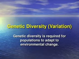
New Concepts Genetic Variation Genetic drift Founder effects Bottleneck effect Mutations Selection Non Random Mating Migration
Genetic Variation Three fundamental levels and each is a genetic resource of potential importance to conservation: • Genetic variation within individuals (heterozygosity) • Genetic differences among individuals within a population • Genetic differences among populations • Species rarely exist as panmictic population = single, randomly interbreeding population • Typically, genetic differences exist among populations—this geographic genetic differences=Crucial component of overall genetic diversity
heterozygosity • Several measures of heterozygosity exist. The value of these measures will range from zero (no heterozygosity) to nearly 1.0 (for a system with a large number of equally frequent alleles). We will focus primarily on expected heterozygosity (HE, or gene diversity, D). The simplest way to calculate it for a single locus is as: • Eqn 4.1where pi is the frequency of the ith of k alleles. [Note that p1, p2, p3 etc. may correspond to what you would normally think of as p, q, r, s etc.]. If we want the gene diversity over several loci we need double summation and subscripting as follows
Heterozygosity • In H.W heterozygosity is given by 2pq. The rest of the expression (p2 + q2) is the homozygosity. • What does heterozygosity tell us and what patterns emerge as we go to multi-allelic systems? Let’s take an example. Say p = q = 0.5. The heterozgosity for a two-allele system is described by a concave down parabola that starts at zero (when p = 0) goes to a maximum at p = 0.5 and goes back to zero when p = 1. In fact for any multi-allelic system, heterozygosity is greatest when • p1 = p2 = p3 = ….pk • The maximum heterozygosity for a 10-allele system comes when each allele has a frequency of 0.1 -- D or HE then equals 0.9. Later, we will see that the simplest way to view FST (a measure of the differentiation of subpopulations) will be as a function of the difference between the Observed heterozygosity, Ho, and the Expected heterozygosity, HE,
Genetic Variation • HT = HP + DPT • where HT = total genetic variation (heterozygosity) in the species; • HP = average diversity within populations (average heterozygosity) • DPT = average divergence among populations across total species range • *Divergence arise among populations from random processes (founder effects, genetic drift, bottlenecks, mutations) and from local selection).
Genetic differentiation • Inbreeding coefficients can be used to measure genetic diversity at different hierachical levels Individual Subpopulation Total population
Wright’s F statistics • Used to measure genetic differentiation • Sometimes called fixation index • Defines reduction in heterozygosity at any one level of population hierachy relative to any other levels: Individual - Subpopulation - Total
Wright’s F statistics • Heterozygosity based on allele frequencies, H = 2pq. • HI, HS, HT refer to the average heterozygosity within individuals, subpopulations and the total population, respectively
Wright’s F statistics • Drop in heterozygosity defined as
Example • 2 subpopulations, gene frequencies p1 = 0.8, p2 = 0.3. • Gene frequency in total population midway between them pt = 0.55 • HS1 = 2p1q1 = 2 x 0.8 x (1-0.8) = 0.32 • HS2 = 2p2q2 = 2 x 0.3 x (1-0.3) = 0.42 • HS = average(HS1,HS2) =(0.32 + 0.42)/2 = 0.37 • HT = 2 x 0.55 x (1 - 0.55) = 0.495
Identity by descent Imagine self-fertilising plant A - A 1,2 - 1,2 | | X ? 1/4 of offspring will be of genotype 1,1 1/2 of offspring will be of genotype 1,2 1/4 of offspring will be of genotype 2,2 FX (inbreeding coefficient) is probability of IBD = 1/2 equivalently, let fAA be the probability of 2 gametes taken at random from A being IBD.
A1A1 A1A2 A1A1 A1A2 A1A2 A2A2 Mutation occurred once • Every mutation creates a new allele • Identity in state = identity by descent (IBD)
A1A1 A1A1 A1A1 A1A2 A1A2 A1A1 A1A2 A1A2 A1A2 A1A2 A2A2 A2A2 A2 A2 IBD A2 A2 IBD A2 A2 alike in state (AIS) not identical by descent The same mutation arises independently
Identity by descent A - B C - D | | P - Q | X Let fAC be the coancestry of A with C etc., i.e. the probability of 2 gametes taken at random, 1 from A and one from B, being IBD. Probability of taking two gametes, 1 from P and one from Q, as IBD, FX
Identity by descent • Example, imagine a full-sib matingA - B / \P - Q | X • Indv. X has 2 alleles, what is the probability of IBD?
Identity by descent • Example, imagine a half-sib matingA - B - C | | P - Q | X
Mutations m=0.0001 A mutates to a at the rate m a reverts back to A at the rate v The equilibrium value for the frequency of A is given by
SNP • Single Nucleotide Polymorphism (SNP) = naturally occuring variants that affect a single nucleotide -predominant form of segregating variation at the molecular level • SNPs are classified according to the nature of the nucleotide that is affected -Noncoding SNP • 5' or 3' nontranscribed region (NTR) • 5' or 3' untranslated region (UTR) • introns • intergenic spacers • Coding SNPs • replacement polymorphisms • synonymous polymorphisms • Transitions [A to G OR C to T] • Transversions [A/G to C/T OR C/T to A/G]
Natural Selection • Tuberculosis (TB) infections have historically swept across susceptible populations killing many. • TB epidemic among Plains Indians of Qu’Appelle Valley Reservation • annual deaths • 1880s 10 % • 1921 7 % • 1950 0.2%
Nonrandom mating • Random mating occurs when individuals of one genotype mate randomly with individuals of all other genotypes. • Nonrandom mating indicates individuals of one genotype reproduce more often with each other • Ethnic or religious preferences • Isolate communities • Worldwide, 1/3 of all marriages are between people born within 10 miles of each other • Cultures in which consanguinity is more prominent • Consanguinity is marriage between relatives • e.g. second or third cousins