Download

1 / 26
270 likes | 428 Vues
Digital Filtering. (1). Difference equation:. (2). Canonical Form:. Digital filtering. u k. y k. The Implementation in MATLAB. Coefficients of numerator and denominator:. Mux – multiplexer DeMux – demultiplexer; ASC- analog signals commutator;

E N D
(1) Difference equation: (2) Canonical Form: Digital filtering uk yk
The Implementation in MATLAB Coefficients of numerator and denominator:
. . Mux – multiplexer DeMux – demultiplexer; ASC- analog signals commutator; ADC, DAC – analog-to-digital and digital-to-analog converters I/O Syst. – “input-output” system CPU – central processor unit CU – control unit ROM – read-only memory RAM – random access memory
(3) Real poles: Complex poles (Second- order-sections (SOS)): (4) (5) (5) The series form of the filter programming: ‑ biquadratic filter ; (5a) + -
. . . x y . . Parallel realization: (6)
FIR and IIR Filters 1.FIR – filters – moving average process (7) (8) Example: Impulse input: Finite impulse response (FIR): 2.IIR – filters – “moving average + auto regression” – ARMA – process. (9)
Impulse Response of the IIR filters (10) (11) b0 = w(0) ; b1- b0a1 = w(1) ; b2- a1b1+b0a21 = w(2) ; ……………………...
Theory of the FIR-filters. w(n-1) w(n) Current data register Convolution processor: Register of constants
0 Types of FIR – filters 3. Band-pass filter (BPF) 2. High-pass filter (HPF) 1. Low-pass filter (LPF) 5. Differentiating filter 6. Integrating filter 4. Band-stop filter (BSF)
Symmetric form of the FIR – filter equation: (1) (2) (2a) (or even filter) Symmetric filter: (2b) (or odd filter) Skew – symmetric filter: For symmetric filter: (3) For skew-symmetric filter: (4)
W(f) 1 Normally: f0=(0.15 : 0.25)fs f -f0 f0 f0 -fs fs -0.5fs 0.5fs Even filter: (5) Low-pass Filters (LPF) Odd filter: (6) Ideal LPF: (7) (8) (9)
W(j) 2=s |W(j)|2 1.4 1.2 1 0.8 0.6 0.4 0.2 0 0 1 2 3 4 5 6 7 2=s =N s/2
N=51 >> b=0.25*sinc(0.25*(-25:25)); >> fvtool(b,1) N=501
Logarithmic Scale N=51 N=501
The Windowing Technique (10) (11) >> b=0.25*sinc(0.25*(-25:25)); >> b=b.*hamming(51); >> fvtool(b,1) Hamming window:
Phase Response 0 -5 Phase (radians) -10 -15 -20 -25 0 0.1 0.2 0.3 0.4 0.5 0.6 0.7 0.8 0.9 p Normalized Frequency ( ґ rad/sample) Linear Phase Response (12) W(z)=W(z-1)(12a) Group delay: (13)
firpm firls %low-pass fir-filters design using different commands n = 20; % Filter order f = [0 0.4 0.5 1]; % Frequency band edges a = [1 1 0 0]; % Desired amplitudes b = firpm(n,f,a); % Design fir-filter using Parks -McClellan algorithm bb = firls(n,f,a); %Design fir-filter using leastsquare method fvtool(b,1,bb,1) % Filter Visualization FIR-filters Design Methods
0 a High –pass (hp) FIR-filters (a) Different FIR-filters Design All-pass (ap) filters: So: b High-pass filters: (14) Band –pass (bp) FIR-filters (b): (15) Band –stop (bs) FIR-filters (c): (16) c
High-pass and Band-stop FIR-filters. %high-pass and bandstop filters n=20; fh = [0 0.7 0.8 1]; % Band edges in pairs ah = [0 0 1 1]; % Highpass filter amplitude fb = [0 0.3 0.4 0.5 0.8 1]; % Band edges in pairs ab = [1 1 0 0 1 1]; % Bandstop filter amplitude bh=firls(n,fh,ah); bs=firls(n,fb,ab); fvtool(bh,1,bs,1)
%multiband fir-filter n=40; f = [0 0.1 0.15 0.25 0.3 0.4 0.45 0.55 0.6 0.7 0.75 0.85 0.9 1]; a = [1 1 0 0 1 1 0 0 1 1 0 0 1 1]; b= firls(n,f,a); fvtool(b,1) Multiband FIR-filter.
n = 20; % Filter order f = [0 0.4 0.5 1]; % Frequency band edges a = [1 1 0 0]; % Desired amplitudes w = [1 10]; % Weight vector b = firpm(n,f,a,w); w1 = [1 2]; b1 = firpm(n,f,a,w1); fvtool(b,1,b1,1) Suppression of Ripples
Differentiators (17) (18) Example: N=3. (19) (20) (21)
bd b Design of Differentiators %differentiators b=firpm(20,[0 0.9],[0 0.9*pi],'d'); bd=firpm(21,[0 1],[0 pi],'d'); fvtool(b,1,bd,1)
%low-pass fir-filters design using different commands n = 50; % Filter order f = [0 0.4 0.5 1]; % Frequency band edges a = [1 1 0 0]; % Desired amplitudes b = firls(n,f,a); [h,t]=stepz(b); [i,t]=impz(b); plot(t,h,'b',t,i,'m'), grid on Impulse and Step Responses