Download
1 / 78
810 likes | 1.11k Vues
Efficient Parallel and Distributed Algorithms for GIS polygon overlay. Satish Puri Dr. Sushil K. Prasad (Chair) Dr. Ying Zhu Dr. Rafal Angryk Dr. Shamkant Navathe. Agenda. Introduction Motivation Goals Result Future work. Polygons. Self-Intersecting polygon.

E N D
Efficient Parallel and Distributed Algorithms for GIS polygon overlay Satish Puri Dr. SushilK. Prasad (Chair) Dr. Ying Zhu Dr. RafalAngryk Dr. ShamkantNavathe
Agenda • Introduction • Motivation • Goals • Result • Future work
Polygons Self-Intersecting polygon
Clipping examples Union Intersection
Polygon Clipping • Input: Given two polygons A = {a1, a2, .. , an} and B = {b1, b2, .. , bm} where ai, bi are vertices represented as (x, y) coordinates and operator ∈ {Union, Intersect, Difference} • Output: C <- AoperatorB
Polygon Overlay • Input: Given two map layers A = {a1, a2, .. , an} and B = {b1, b2, .. , bm} where ai, bi are polygons represented as (x,y) coordinates of vertices and operator op∈ {Union, Intersect, Difference} • Output: C <- AopB
Geographic Information System (GIS) Application • Map of population distribution • Map of a region affected by • hurricane Sandy Where are the safe rescue shelters?
Applications • GIS Polygon overlay • Computer Graphics – zooming an image, image rendering in 3D graphics, video games • VLSI CAD design rule checking, layout verification
VLSI CAD Applications • intersection and union for PCB power integrity analysis Figure: Small clip from one layer of a microprocessor package layout
Challenges • Size of data (GIS:100k vertices, GBs) • Excessive runtime eg: Large scale polygon clipping at Intel - some clippers took several days on a one-terabyte memory server - Best polygon clipper took 4.5 hours on a Xeon 3.0 GHz workstation with 32 GB of RAM. • Excessive memory consumption
Goals • Output-Sensitive Parallel Algorithms for clipping a pair of polygons • Parallel Polygon Overlay using shared memory • Distributed Polygon Overlay using cluster
Goal 1 Output-Sensitive Parallel Algorithms for clipping a pair of polygons • Parallelization of plane-sweep based algorithm • Parallelization of graph-traversal based algorithm • Complexity Analysis using PRAM model • Parallel Segment tree data structure construction • Segment tree based polygon clipping algorithm
Motivation • Lack of output-sensitive parallel algorithm for polygon clipping O(log n) using O(n2) processors [1] • Lack of multi-threaded algorithm for clipping arbitrary polygons on CPU/GPU • Existing parallel algorithms do not support arbitrary polygons (self-intersecting)
Publications • Satish Puri and Sushil K. Prasad, "Output-Sensitive Parallel Algorithm for Polygon Clipping", International Conference on Parallel Processing, ICPP, 2014
Intersections (k): Output-Sensitive kis number of intersection, N is edges1. For polygons with m and n vertices,Brute force algorithm = O(mn) 2. Self-intersecting: O(m2 + n2 + mn)
Output-sensitive algorithm • The asymptotic running time of algorithm always input-sensitive (depends on n) Output-sensitive: • If the output is large, brute force algorithm is fine, but • If output is small, we want a fast algorithm
Output-Sensitive Parallel Algorithms • number of processors vary based on output size • e.gcomputing the intersections of n edges: the time and number of processors used may depend on n as well as the number of the actual intersections (k)
Existing parallel output-sensitive algorithms • Line segment intersection reporting in parallel Rub: O(((n + k) lognloglogn)/p), using procs p<=(n+k) • Intersecting line segments in parallel using output-sensitive number of processors Goodrich: O(log2n) time using O(n + k/log n) processors
PRAM Polygon Clipping c7 s4 Output-Sensitive Algorithms: • O(log n) time algorithm using plane sweep method using O(n+k+k’) processors • O(log n) time algorithm using graph traversal method with O(n+ k) processors in PRAM model where n = polygon edges k = edge intersections k’ = additional vertices due to partitioning c6 s5 s3 I8 c8 c5 s6 I7 I6 I5 c4 I4 I3 c3 c9 I1 I2 s7 c2 s1
Comparing with literature Literature [1] A parallel algorithm for computing polygon set operations, Parallel Processing Symposium, 1994 [2] Efficient clipping of arbitrary polygons, ACM Transactions on Graphics, 1998 [3] Industrial strength polygon clipping: A novel algorithm with applications in VLSI CAD, Computer-Aided Design, 2010 [4] A generic solution to polygon clipping, Communications of the ACM, 1992
Computation Involved • Input: Polygons P1 and P2 with n and m edges 1) finding edge intersections, O(mn) 2) classifying input vertices as contributing or non-contributing to output, O(n) 3) stitching together the vertices generated in Step 1 and 2 to produce one or more output polygons.
Sequential Clipping Example c7 s4 c6 s5 s3 I8 c8 c5 s6 I7 I6 I5 c4 I4 I3 c3 c9 I1 I2 s7 c2 s1 c1
Sequential Clipping Example c7 s4 c6 s5 s3 I8 c8 c5 s6 I7 I6 I5 c4 I4 I3 c3 c9 I1 I2 s7 s7 c2 s1 s1 c1
Sequential Clipping Example c7 s4 c6 s5 s3 I8 c8 c5 s6 I7 I6 I5 c4 I4 I3 c3 c9 I1 I2 s7 s7 c2 s1 s1 c1
Sequential Clipping Example c7 s4 c6 s5 s3 I8 c8 c5 s6 I7 I6 I5 c4 I4 I3 c3 c9 I1 I2 s7 s7 c2 s1 s1 c1
Sequential Clipping Example c7 s4 c6 s5 s3 I8 c8 c5 s6 I7 I6 I5 c4 I4 I3 c3 c9 I1 I2 s7 s7 c2 s1 s1 c1
Sequential Clipping Example c7 s4 c6 s5 s3 I8 c8 c5 s6 I7 I6 I5 c4 I4 I3 c3 c9 I1 I2 s7 s7 c2 s1 s1 c1
Sequential Clipping Example c7 s4 s4 c6 s5 s5 s3 I8 I8 c8 c5 s6 I7 I7 I6 I6 I5 I5 c4 c4 I4 I4 I3 I3 c3 c9 I1 I2 I1 I2 s7 s7 c2 s1 s1 c1
Parallel processing of a scanbeam c7 s4 c6 s5 s3 I8 s6’ s6 c8 c5 s6 I6 I7 I7 I6 I5 Scan beam I5 c4 I4 c4’ c4 I3 c3 c9 I1 I2 s7 c2 s1
Lemma Scan beam s6’ s6 I6 I7 I5 The polygon edges in a scanbeamcan be labeled as left or right without looking at the overall geometry and the labels alternate one another. A vertex can be classified as contributing or not independently in a scanbeam. Contributing Vertices in O(logn)time. The number of intersections in a scanbeamcan be computed in O(logn) time using O(n)processors c4’ c4
Intersections = Inversions Inversion: a pair which is not in sorted order Array A, index i and j i<j and A[i] > A[j] Unordered: 3, 2, 4, 1 Inversions: (3,1), (3,2), (4,1), (2,1) Fig. Intersection of 4 edges in a scanbeam
Counting Inversions while merging A = {A1, A2, .., An} Al = {A1, A2, .., Amid} Ar = {Amid+1, Amid+2, .., An} Suppose ai > aj Inversions: (ai,aj), (ai+1,aj), .., (amid,aj) Bigger than aj ai aj
s4 s5’ s5 c7 s5’ s5 s4 s3 c6 I8 s5 s3 s6 s6’ I8 c8 s6 s6’ c5 s6 I6 I7 I7 I6 I5 I5 c4 c4 c4’ I4 c4’ c4 I3 I4 c3 c3 I3 c9 I1 I2 I2 s7 I1 c2 s1 s7 s7’ s7 s7’ c1
s4 s’5s4s5 s5’ s5 s’5s4s5I8s6’s6I8s3 s5I8s6’s6I8s3s5’ s5’ s4 s5 s6I8s3s5’ s4s5I8s6’ I8 s3 s6’ s6 s5 s6I8s3s4s5I8 I7I5c4I3 I4I5I6 (P2) s3 s6 s6’ I8 s6 I5 I6 I7 I7 s6’I7I5 c4I3 I4c4’I5I6s6 I6 c4’ c4 c4’I5I6s6s6’I7I5c4 c4’I5I6s6s6’I7I5I3 I4 I5 c4 c4 I3 I4c4’ I4 c4’ I4 c4 I3 I3 I2 I1 I2 I1 s7 s7 s7’ s7I2I1s7’ s1 s7I2I1s1 (P1) s7’s1s7 s7 s7’ s1
Parallel algorithm based on Greiner-Hormann Algorithm c7 s4 c6 s5 s3 I8 c8 c5 s6 I7 I6 I5 s2 c4 I4 I3 c3 c3 I2 c9 I1 s7 Polygon 1: I1 S1 S7 I2 Polygon 2: I3 I4 I7 S3 S4 S5 S6 I6 C4 c2 s1 c1
Segment tree based polygon clipping • Parallel constuction • Intersection computation
7 1 g Polygon A: {a, b,.., g} Polygon B: {1, 2,.. 7} Segment Tree O(log n) construction using n processors Cover list: CA and CB O(log n + k) for point query k is the number of retrieved segments a 6 f b 5 e 2 c 3 d 4
7 1 g a 6 f b 5 e 2 Polygon A: {a, b,.., g} Polygon B: {1, 2,.. 7} Segment Tree with cover list (C) and end list (E) Finding intersections a ∈ CA and b ∈ CB a∈ CA and b ∈ EB a∈ EA and b ∈ CB c 3 d 4
Goal 2 Parallel polygon overlay using shared memory • P-thread based implementation for overlaying two layers of polygons. (b) Multi-threaded implementation of Vatti's algorithm and Greiner-Hormann's algorithm. (c) CUDA (GPU) based design and implementation for overlaying two layers of polygons.
Current work • Parallelized Vatti’s Polygon Clipping algorithm - for a pair of polygon (Java Threads) - for two sets of real-world polygons using P-Threads
Experimental Setup • 64-bit CentOSoperating system running on AMD Opteron • Processor 6272 (1.4 GHz) with 64 CPU cores • 64 GB memory
Simulated data Fig.Performance of multi-threaded algorithm for with different output sizes shown in thousands (k) of edges.
Real-world data Performance impact of varying number of threads for real-world datasets for Intersection and Union operation