Download

1 / 25
360 likes | 894 Vues
DCT. lecture6. 3. Discrete Cosine transform (DCT). The discrete cosine transform (DCT) is the basis for many image compression algorithms they use only cosine function only. Assuming an N*N image , the DCT equation is given by. In matrix form for DCT the equation become as.

E N D
DCT lecture6
3. Discrete Cosine transform (DCT) The discrete cosine transform (DCT) is the basis for many image compression algorithms they use only cosine function only. Assuming an N*N image , the DCT equation is given by In matrix form for DCT the equation become as where u= 0,1,2,…N-1 along rows and v= 0,1,2,…N-1 along columns
Properties of DCT • One clear advantage of the DCT over the DFT is that there is no need to • manipulate complex numbers. • the DCT is designed to work on pixel values ranging from -0.5 to 0.5 for binary image and from -128 to 127 for gray or color image so the original image block is first “leveled off” by subtract 0.5 or 128 from each entry pixel values. the general transform equation for DCT is Original image DCT
Derive the DCT coefficient matrix of 4 * 4 block image v0 v1 v2 v3 u0 u1 u2 u3
EX1: Calculate the DCT transform for the image I(4,4) D I D I D I
So the (DCT) matrix of 8*8 image inverse discrete cosine transform (IDCT) the general inverse transform equation for DCT is
wavelet Lecture 6
Filtering After the image has been transformed into the frequency domain , we may want to modify the resulting spectrum 1. high-pass filter:-use to remove the low- frequency information which will tend to sharpen the image 2. low-pass filter:-use to remove the high- frequency information which will tend to blurring or smoothing the image 3. Band-pass filter:-use to extract the(low , high) frequency information in specific parts of spectrum 4. Band-reject:-use to eliminate frequency information from specific part of the spectrum
4. Discrete wavelet transform (DWT) Definition:-The wavelet transform is really a family transform contains not just frequency information but also spatial information Numerous filters can be used to implement the wavelet transform and the two commonly used are the Haar and Daubechies wavelet transform . Wavelet families Haar wavelet Daubechies families (D2,D3,D4,D5,D6,…..,D20) biorthogonal wavelet Coiflets wavelet Symlets wavelet Morlet wavelet
The discrete wavelet transform of signal or image is calculated by passing it through a series of filters called filter bank which contain levels of low-pass filter (L) and high- pass (H) simultaneously . They can be used to implement a wavelet transform by first convolving them with rows and then with columns. The outputs giving the detail coefficients (d) from the high-pass filter and course approximation coefficients (a) from the low-pas filter . Implement DWT:- decomposition algorithm Convolve the low-pass filter with the rows of image and the result is (L) band with size (N/2,N). 2. Convolve the high-pass filter with the rows of image and the result is (H) band with size (N/2,N).
Convolve the columns of (L) band with low-pass filter and the result is (LL) band with size (N/2,N/2). • Convolve the columns of (L) band with high-pass filter and the result is (LH) band with size (N/2,N/2). • Convolve the columns of (H) band with low-pass filter and the result is (HL) band with size (N/2,N/2). • Convolve the columns of (H) band with high-pass filter and the result is (HH) band with size (N/2,N/2).
This six steps of wavelet decomposition are repeated to further increase the detailed and approximation coefficients decomposed with high and low pass filters . in each level we start from (LL) band . the DWT decomposition of input image I(N,N) show as follow for two levels of filter bank column column rows rows Level 1 (N/2, N/2) Level 2 (N/4*N/4)
Haar wavelet transform The Haar equation to calculate the approximation coefficients and detailed coefficients given as follow if si represent the input vector Low –pass filter for Haar wavelet L0 = 0.5 L1= 0.5 high–pass filter for Haar wavelet H0 = 0.5 H1= - 0.5 approximation coefficients detailed coefficients Calculate the Haar wavelet for the following image
117 101 104 138 161 152 170 132 120 111 125 143 154 154 151 136 113 144 140 162 168 179 184 151 108 151 156 181 159 145 152 134 I= 110 151 154 135 114 95 100 121 135 169 134 108 107 110 112 147 149 150 125 132 129 156 163 159 135 107 132 149 141 150 135 156 L H 151 109 156.5 121 8 -17 4.5 19 143.5 115.5 154 134 4.5 -9 0 7.5 167.5 128.5 173.5 151 -15.5 -11 -5.5 16.5 143 129.5 152 168.5 -21.5 -12.5 7 9 110.5 130.5 104.5 144.5 -20.5 9.5 9.5 -10.5 129.5 152 108.5 121 -17 13 -1.5 -17.5 161 149.5 142.5 129.5 -0.5 -2.5 -13.5 2 145 121 145.5 140.5 14 -8.5 -4.5 10.5
Then convolution the columns of result with low and high -pass filters L H 1 1 151 109 156.5 121 8 -17 4.5 19 143.5 115.5 154 134 4.5 -9 0 7.5 167.5 128.5 173.5 151 -15.5 -11 -5.5 16.5 143 129.5 152 168.5 -21.5 -12.5 7 9 110.5 130.5 104.5 144.5 -20.5 9.5 9.5 -10.5 129.5 152 108.5 121 -17 13 -1.5 -17.5 161 149.5 142.5 129.5 -0.5 -2.5 -13.5 2 145 121 145.5 140.5 14 -8.5 -4.5 10.5 112.25 127.5 155.25 147.25 6.25 2.25 -13 13.25 159.75 129 155.25 162.75 -18.5 0.75 -11.75 12.75 120 106.5 141.25 132.75 4 -18.75 11.25 -14 144 153.25 6.75 -9 -5.5 135.25 135 6.25 1 1 1.25 -6.5 -3.25 5.75 3.75 1.75 -4 2.25 10.75 -8.75 -0.5 12.25 3 -6.25 0.75 3.75 11.75 -9.5 -10.75 -2 -1.75 -1.75 5.5 3.5 14.25 7.75 -7,75 -4.5 3 -4.25 -1.5 -5.5
in the next level we start with (LL1) band 1 112.25 127.5 155.25 147.25 129 159.75 155.25 162.75 120 106.5 132.75 141.25 144 153.25 135.25 135 After apply convolution rows of (LL1) band with law-pass ,high pass filters L2 H2 119.875 -7.625 4 151.25 144.375 3.75 -15.375 159 137 113.25 4.24 -6.75 135.125 148.75 0.125 -4.625 Then convolution the columns of result with low and high -pass filters LL2 HL2 132.125 155.125 -11.5 3.875 136.062 130.937 -5.687 2.1875 -12.25 -3.875 3.875 0.125 -17.687 2.0625 -1.062 0.9375 LH2 HH2
So the decomposition for two levels are 1 2.25 6.25 -13 13.25 LL2 HL2 0.75 -18.5 -11.75 12.75 155.125 132.125 -11.5 3.875 4 -18.75 11.25 -14 136.062 130.937 -5.687 2.1875 -9 6.75 -5.5 6.25 -12.25 -3.875 0.125 3.875 -17.687 -1.062 2.0625 0.9375 HH2 LH2 5.75 -6.5 -3.25 3.75 1.75 -4 2.25 1.25 -8.75 -6.25 3 0.75 3.75 -0.5 12.25 10.75 -1.75 -1.75 5.5 3.5 11.75 -9.5 -10.75 -2 1 1 -7,75 -4.5 3 -4.25 14.25 7.75 -1.5 -5.5
inverse Haar wavelet transform To reconstructs the original image we use the following equations First begin with (LL2) band and apply the above equations with each corresponded element of (HL2) band rows , and the same work apply between LH2 and HH2 rows LL2 HL2 132.125 155.125 -11.5 3.875 136.062 130.937 2.1875 -5.687 -12.25 -3.875 3.875 0.125 0.9375 -17.687 2.0625 -1.062 LH2 HH2 120.625 143.625 159 151.25 138.25 133.874 125.25 136.624 -8.375 -16.125 -3.75 -4 3 -1.125 -18.749 -16.625
Then apply the above equations with columns of new matrix as showing 1 120.625 159 151.25 143.625 138.25 125.25 136.624 133.874 -8.375 -3.75 -4 -16.125 3 -18.749 -16.625 -1.125 127.5 155.25 147.25 112.25 159.75 162.75 155.25 129 120 141.25 132.75 106.5 135.25 135 144 153.25
112.25 127.5 155.25 147.25 1 6.25 2.25 -13 13.25 1 159.75 129 155.25 162.75 -18.5 0.75 -11.75 12.75 120 4 -18.75 11.25 106.5 -14 141.25 132.75 6.75 -9 -5.5 144 153.25 6.25 135.25 135 5.75 1.75 -4 2.25 1.25 -6.5 -3.25 3.75 3 -6.25 0.75 3.75 10.75 -8.75 -0.5 12.25 -1.75 -1.75 5.5 3.5 11.75 -9.5 -10.75 -2 -7,75 -4.5 3 -4.25 14.25 7.75 -1.5 -5.5 153 157.5 160.5 134 118.5 106 114.5 140.5 1 1
153 157.5 160.5 134 118.5 106 114.5 140.5 162 163.5 168 142.5 110.5 147.5 148 171.5 102.5 110.5 106 134 122.5 160 144 121.5 153 135 159.5 147 142 128.5 129.5 140.5 -1 3.5 9.5 -2 -1.5 -5 -10.5 -2.5 17 4.5 16 8.5 2.5 -3.5 -8 -9.5 -7.7 3.5 -6 -13 -12.5 -9 10 13.5 3 -6 3.5 12 6.5 22 -2.5 -8.5 117 120 113 108
117 101 104 138 161 152 170 132 120 111 125 143 154 154 151 136 113 144 140 162 168 179 184 151 108 151 156 181 159 145 152 134 Home work I= 110 151 154 135 114 95 100 121 135 169 134 108 107 110 112 147 149 150 125 132 129 156 163 159 135 107 132 149 141 150 135 156 I=