Download
1 / 38
380 likes | 560 Vues
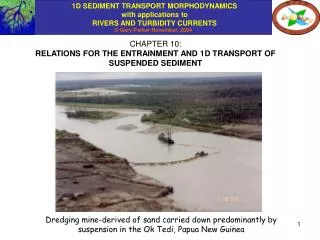
CHAPTER 10: RELATIONS FOR THE ENTRAINMENT AND 1D TRANSPORT OF SUSPENDED SEDIMENT . Dredging mine-derived of sand carried down predominantly by suspension in the Ok Tedi, Papua New Guinea. THE STRATEGY.

E N D
CHAPTER 10: RELATIONS FOR THE ENTRAINMENT AND 1D TRANSPORT OF SUSPENDED SEDIMENT Dredging mine-derived of sand carried down predominantly by suspension in the Ok Tedi, Papua New Guinea
THE STRATEGY Consider the case of an equilibrium suspension in an equilibrium (normal) 1D open channel flow. Returning to the equation of conservation of suspended sediment from Chapter 4, • Under equilibrium conditions the dimensionless entrainment rate E is equal to the near-bed average concentration of suspended sediment! We can: • Obtain empirical relation for E versus boundary shear stress for equilibrium conditions. • With luck, the relation can be applied to conditions that are not too strongly disequilibrium.
THE STRATEGY contd. • For equilibrium open-channel suspensions, • Determine a position z = b near the bed and measure the volume concentration • of suspended sediment averaged over turbulence there. Note that the definition of b is peculiar to each researcher, but in general b/H << 1. • Determine the boundary shear stress b, or if bedforms are present the component due to skin friction bs. Here we use the notation bs so as to always admit the possibility of form drag. • 3. If the sediment can be approximated as uniform with size D, compute s* = • bs/(RgD) and plot E versus s* to determine an entrainment rate. • If the sediment is to be treated as a mixture of sizes Di with fractions Fi in the • bed surface layer, from the measured entrainment rates Ei determine the • entrainment rates per unit content in the surface layer Eui = Ei/Fi, and plot Eui • versus si* = bs/(RgDi).
ENTRAINMENT RELATIONS FOR UNIFORM MATERIAL Garcia and Parker (1991) reviewed seven entrainment relations and recommended three of these; Smith and McLean (1977), van Rijn (1984) and (surprise surprise) Garcia and Parker (1991). Smith and McLean (1977) offer the following entrainment relation. The reference height is evaluated at what the authors describe as the top of the bedload layer; where ks denotes the Nikuradse roughness height, The authors give no guidance for the choice of bc. It is suggested here that it might be computed as bc=RgDc*, where c* is given by the Brownlie (1981) fit to the Shields relation:
ENTRAINMENT RELATIONS FOR UNIFORM MATERIAL contd. The entrainment relation of van Rijn (1984) takes the form The reference level b is set as follows: b = 0.5 b, where b = average bedform height, when known; b = the larger of the Nikuradse roughness height ks or 0.01 H when bedforms are absent or bedform height is not known. The critical Shields number can be evaluated with the Brownlie (1981) fit to the Shields curve:
ENTRAINMENT RELATIONS FOR UNIFORM MATERIAL contd. Garcia and Parker (1991) use a reference height b = 0.05 H; Wright and Parker (2004) found that the relation of Garcia and Parker (1991) performs well for laboratory flumes and small to medium sand-bed streams, but does not perform well for large, low-slope streams. Wright and Parker (2004) have thus amended the relationship to cover this latter range as well Again the reference height b = 0.05 H. This corrects Garcia and Parker to cover large, low-slope streams:
ENTRAINMENT RELATIONS FOR SEDIMENT MIXTURES Garcia and Parker (1991) generalized their relation to sediment mixtures. The relation for mixtures takes the form where Fi denotes the fractions in the surface layer and denotes the arithmetic standard deviation of the bed sediment on the scale. The reference height b is again equal to 0.05 H. Wright and Parker (2004) amended the above relation so as to apply to large, low-slope sand bed rivers as well as the types previously considered by Garcia and Parker (1991). The relation is the same as that of Garcia and Parker (1991) except for the following amendments:
ENTRAINMENT RELATIONS FOR SEDIMENT MIXTURES contd. McLean (1992; see also 1991) offers the following entrainment formulation for sediment mixtures. Let ET denote the volume entrainment rate per unit bed area summed over all grain sizes, pi denote the fractions in the ith grain size range in the bedload transport and psbi = Ei/ET denote the fractions in the ith grain size range in the sediment entrained from the bed. Then where p denotes bed porosity, The critical boundary shear stress bc is evaluated using bed material D50; again the Brownlie (1981) fit to the Shields curve is suggested here.
LOCAL EQUATION OF CONSERVATION OF SUSPENDED SEDIMENT Once entrained, suspended sediment can be carried about by the turbulent flow. Let c denote the instantaneous concentration of suspended sediment, and (u, v, w) denote the instantaneous flow velocity vector. The instantaneous velocity vector of suspended particles is assumed to be simply (u, v, w - vs) where vs denotes the terminal fall velocity of the particles in still water. Mass balance of suspended sediment in the illustrated control volume can be stated as or thus
AVERAGING OVER TURBULENCE In a turbulent flow, u, v, w and c all show fluctuations in time and space. To represent this, they are decomposed into average values (which may vary in time and space at scales larger than those characteristic of the turbulence) and fluctuations about these average values. By definition, then, The equation of conservation of suspended sediment mass is now averaged over turbulence, using the following properties of ensemble averages: a) the average of the sum = the sum of the average and b) the average of the derivative = the derivative of the average, or
AVERAGING OVER TURBULENCE contd. Recalling that vs is a constant, substituting the decompositions into the equation of mass conservation of suspended sediment results in Now for example so that the final form of the averaged equation is
LOCAL STREAMWISE MOMENTUM CONSERVATION The convective flux of any quantity is the quantity per unit volume times the velocity it is being fluxed. So, for example, the convective flux of streamwise momentum in the upward direction is wu = wu. The viscous shear stress acting in the x (streamwise) direction on a face normal to the z (upward) direction is The balance of streamwise momentum in the control volume requires that: (streamwise momentum)/t = net convective inflow of momentum + net shear force + net pressure force + downslope force of gravity
LOCAL STREAMWISE MOMENTUM CONSERVATION contd. A reduction yields the relation Averaging over turbulence in the same way as before yields the result where Here denotes the z-x component of the Reynolds stress generated by the turbulence; the term is known as the Reynolds flux of streamwise momentum in the upward direction. For fully turbulent flow, the Reynolds stress Rzx is usually far in excess of the viscous stress , which can be dropped.
LOCAL STREAMWISE MOMENTUM CONSERVATION FOR NORMAL FLOW The shear Reynolds stress Rzx is abbreviated as ; its value at the bed is b.. When the flow is steady and uniform in the x and y directions, streamwise momentum balance becomes or thus Integrating this equation under the condition of vanishing shear stress at the water surface z = H yields the result Depth-slope product! Linear distribution of shear stress!
REYNOLDS FLUX OF SUSPENDED SEDIMENT The terms denote convective Reynolds fluxes of suspended sediment. They characterize the tendency of turbulence to mix suspended sediment from zones of high concentration to zones of low concentration, i.e. down the gradient of mean concentration. In the case illustrated below concentration declines in the positive z direction; turbulence acts to mix the sediment from the zone of high concentration (low z) to the zone of low concentration (high z).
REYNOLDS FLUX OF STREAMWISE MOMENTUM The shear stress , or equivalently the Reynolds flux of streamwise (x) momentum in the upward (z) direction characterizes the tendency of turbulence to transport streamwise momentum from high concentration to low. In the case of open channel flow, the source for streamwise momentum is the downstream gravity force term gS. This momentum must be fluxed downward toward the bed and exited from the system (where the loss of momentum is manifested as a resistive force balancing the downstream pull of gravity) in order to achieve momentum balance. This downward flux is maintained by maintaining a streamwise momentum profile that has high velocity in the upper part of the flow and low velocity in the lower part of the flow. This in turn generates a negative value of and a positive value of .
REPRESENTATION OF REYNOLDS FLUX WITH AN EDDY DIFFUSIVITY The concentration of any quantity in a flow is the quantity per unit volume. Thus the concentration of streamwise momentum in the flow is u and the volume concentration of suspended sediment is c. The tendency for turbulence to mix any quantity down its concentration gradient (from high concentration to low concentration) can be represented in terms of a kinematic eddy diffusivity: Reynolds flux of suspended sediment in the z direction: Reynolds flux of streamwise momentum in the z direction: In the above relations st is the kinematic eddy diffusivity of suspended sediment [L2/T] and t is the kinematic eddy diffusivity (eddy viscosity) of momentum.
EDDY VISCOSITY FOR TURBULENT OPEN CHANNEL FLOW The standard equilibrium velocity profile for hydraulically rough turbulent open-channel flow is the logarithmic profile; where = 0.4 and u* = (gHS)1/2. The eddy diffusivity of momentum can be back-calculated from this equation; Solving for t, a parabolic form is obtained; or
EQUILIBRIUM VERTICAL DISTRIBUTION OF SUSPENDED SEDIMENT According to the Reynolds analogy, turbulence transfers any quantity, whether it be momentum, heat, energy, sediment mass, etc. in the same fundamental way. While it is an approximation, it is a good one over a relatively wide range of conditions. As a result, the following estimate is made for the eddy diffusivity of sediment: For steady flows that are uniform in the x and z directions maintaining a suspension that is similarly steady and uniform, the equation of conservation of suspended sediment reduces to
EQUILIBRIUM SUSPENSIONS contd. The balance equation of suspended sediment thus becomes This equation can be integrated under the condition of vanishing net sediment flux in the z direction at the water surface to yield the result i.e. the upward flux of suspended driven by turbulence from high concentration (near the bed) to low concentration (near the water surface) is perfectly balanced by the downward flux of suspended sediment under its own fall velocity. The Reynolds flux F can be related to the gradient of the mean concentration as The balance equation thus reduces to:
SOLUTION FOR THE ROUSE-VANONI PROFILE The balance equation is: The boundary condition on this equation is a specified upward flux, or entrainment rate of sediment into suspension at the bed: Rouse (1939) solved this problem and obtained the following result, which is traditionally referred to as the Rouse-Vanoni profile.
REFERENCE LEVEL The reference level cannot be taken as zero. This is because turbulence cannot persist all the way down to a solid wall (or sediment bed). No matter whether the boundary is hydraulically rough or smooth, essentially laminar effects must dominate right near the wall (bed). It is for this reason that the logarithmic velocity law yields a value for of - at z = 0. The point of vanishing velocity is reached at z = ks/30. Since the eddy diffusivity from which the profile of suspended sediment is computed was obtained from the logarithmic profile, it follows that cannot be computed down to z = 0 either. The entrainment boundary condition must be applied at z = b ks/30.
AND NOW IT’S TIME FOR SPREADSHEET FUN!! Go toRTe-bookRouseSpreadsheetFun.xls This spreadsheet allows calculation of the suspended sediment profile from specified values of b/H, vs and u* using the Rouse-Vanoni profile.
1D SUSPENDED SEDIMENT TRANSPORT RATE FROM EQUILIBRIUM SOLUTION The volume suspended sediment transport rate per unit width is qs computed as In order to perform the calculation, however, it is necessary to know the velocity profile over a bed which may include bedforms. This velocity profile may be specified as where kc is a composite roughness height. If bedforms are absent, kc = ks = nkDs90. If bedforms are present, the total friction coefficient Cf = Cfs + Cff may be evaluated (using a resistance predictor for bedforms if necessary) and kc may be back-calculated from the relation
1D SUSPENDED SEDIMENT TRANSPORT RATE FROM EQUILIBRIUM SOLUTION It follows that qs is given by the relations The integral is evaluated easily enough using a spreadsheet. This is done in the next chapter.
CLASSICAL CASE OF DISEQUILIBRIUM SUSPENSION: THE 1D PICKUP PROBLEM Consider a case where sediment-free equilibrium open-channel flow over a rough, non-erodible bed impinges on an erodible bed offering the same roughness. • The flow can be considered quasi-steady over time spans shorter than that by which significant bed degradation occurs. • The flow but not the suspended sediment profile can be considered to be at equilibrium.
THE 1D PICKUP PROBLEM contd. Governing equation Boundary conditions Can be used to find adaptation length Lsr for suspended sediment Solution yields the result that A method for estimating Lsr is given in Chapter 21.
WHICH VERSION OF THE EXNER EQUATION OF BED SEDIMENT CONTINUITY SHOULD BE USED FOR A MORPHODYNAMIC PROBLEM CONTROLLED BY SUSPENDED SEDIMENT? Should the formulation be with E computed based on local flow conditions, or with qs computed from the quasi-equilibrium relation applied to local flow conditions? The answer depends on the characteristic length L of the phenomenon of interest (one meander wavelength, length of alluvial fan etc.) compared to the adaptation length Ls required for the flow to reach a quasi-equilibrium suspension. If L < Ls the former formulation should be used. If L > Ls the latter formulation can be used. Selenga Delta, Lake Baikal, Russia: image from NASA https://zulu.ssc.nasa.gov/mrsid/mrsid.pl
SELF-STRATIFICATION OF THE FLOW DUE TO SUSPENDED SEDIMENT A flow is stably stratifiedif heavier fluid lies below lighter fluid. The density difference suppresses turbulent mixing. The city of Phoenix, Arizona, USA during an atmospheric inversion Sediment-laden flows are self-stratifying Well, somewhere down there Here susp = density of the suspension and e = fractional excess density due to the presence of suspended sediment.
FLUX AND GRADIENT RICHARDSON NUMBERS The damping of turbulence due to stable stratification is controlled by the flux Richardson number Rif. [Rate of expenditure of turbulent kinetic energy in holding the (heavy) sediment in suspension]/[Rate of generation of turbulent kinetic energy by the flow] Turbulence is not suppressed at all for Rif = 0. Turbulence is killed completely when Rif reaches a value near 0.2 (e.g. Mellor and Yamada, 1974) Now let where Ri denotes the gradient Richardson Number Then
SUSPENSION WITH SELF-STRATIFICATION: SMITH-MCLEAN FORMULATION Smith and McLean (1977), for example, propose the following relation for damping of mixing due to self-stratification: The balance equations and boundary conditions take the forms: These relations may be solved iteratively for concentration and velocity profiles in the presence of stratification.
SUSPENSION WITH SELF-STRATIFICATION: GELFENBAUM-SMITH FORMULATION The workbook RTe-bookSuspSedDensityStrat.xls implements the formulation for stratification-mediated suppression of mixing due to Gelfenbaum and Smith (1986); It also uses the specification b = 0.05 H. The balance equations and boundary conditions take the forms: These relations may be solved iteratively for concentration and velocity profiles in the presence of stratification. The workbook RTe-bookSuspSedDensityStrat.xls provides a numerical implementation.
ITERATION SCHEME The governing equations for flow velocity and suspended sediment concentration can be integrated to give the forms where The relations of the previous slide can be rearranged to give The iteration scheme is commenced with the logarithmic velocity profile for velocity and the Rouse-Vanoni profile for suspended sediment: where the superscript (0) denotes the 0th iteration (base solution).
ITERATION SCHEME contd. The iteration then proceeds as Iteration continues until is tolerably close to and is tolerably close to . A dimensionless version of the above scheme is implemented in the workbook Rte-bookSuspSedDensityStrat.xls. Moredetails about the formulation are provided in the document Rte-bookSuspSedStrat.doc.
INPUT VARIABLES FOR Rte-bookSuspSedDensityStrat.xls The first step in using the workbook is to input the parameters R+1 (sediment specific gravity), D (grain size), H (flow depth), kc (composite roughness height including effect of bedforms, if any), u (shear velocity) and (kinematic viscosity of water). When bedforms are absent, the composite roughness height kc is equal to the grain roughness ks. In the presence of bedforms, kc is predicted from one of the relations of Chapter 9 and the equations The user must then click a button to clear any old output. After this step, the user is presented with a choice. Either the near-bed concentration of suspended sediment can be specified by the user, or it can be calculated from the Garcia-Parker (1991) entrainment relation. In the former case, a value for must be input. In the latter case, a value for the shear velocity due to skin friction us must be input. It follows that in the latter case us can be predicted using one of the relations of Chapter 9. Once either of these options are selected and the appropriate data input, a click of a button performs the iterative calculation for concentration and velocity profiles. Note: the iterative scheme may not always converge!
SAMPLE CALCULATION (a) with Garcia-Parker entrainment relation qs with stratification = 0.72 x qs without stratification Stratification neglected Stratification included Stratification included Stratification neglected
SAMPLE CALCULATION (b) with Garcia-Parker entrainment relation qs with stratification = 0.39 x qs without stratification Stratification neglected Stratification included Stratification included Stratification neglected
REFERENCES FOR CHAPTER 10 Brownlie, W. R., 1981, Prediction of flow depth and sediment discharge in open channels, Report No. KH-R-43A, W. M. Keck Laboratory of Hydraulics and Water Resources, California Institute of Technology, Pasadena, California, USA, 232 p. García, M., and G. Parker, 1991, Entrainment of bed sediment into suspension, Journal of Hydraulic Engineering, 117(4): 414-435. Gelfenbaum, G. and Smith, J. D., 1986, Experimental evaluation of a generalized suspended-sediment transport theory, in Shelf and Sandstones, Canadian Society of Petroleum Geologists Memoir II, Knight, R. J. and McLean, J. R., eds., 133 – 144. McLean, S. R., 1991, Depth-integrated suspended-load calculations, Journal of Hydraulic Engineering, 117(11): 1440-1458. McLean, S. R., 1992, On the calculation of suspended load for non-cohesive sediments, 1992, Journal of Geophysical Research, 97(C4), 1-14. Mellor, G. and Yamada, T., 1974, A hierarchy of turbulence closure models for planetary boundary layers: Journal of Atmospheric Science, v.31, 1791-1806. van Rijn, L. C., 1984, Sediment transport. II: Suspended load transport Journal of Hydraulic Engineering, 110(11), 1431-1456. Rouse, H., 1939, Experiments on the mechanics of sediment suspension, Proceedings 5th International Congress on Applied Mechanics, Cambridge, Mass,, 550-554. Smith, J. D. and S. R. McLean, 1977, Spatially averaged flow over a wavy surface, Journal of Geophysical Research, 82(12): 1735-1746. Wright, S. and G. Parker, 2004, Flow resistance and suspended load in sand-bed rivers: simplified stratification model, Journal of Hydraulic Engineering, 130(8), 796-805.