Download
1 / 57
660 likes | 1k Vues
Chap 5. Identical Particles. Two-Particle Systems Atoms Solids Quantum Statistical Mechanics. Two particles having the same physical attributes are equivalent . They behave the same way if subjected to the same treatment.

E N D
Chap 5. Identical Particles Two-Particle Systems Atoms Solids Quantum Statistical Mechanics
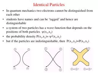
Two particles having the same physical attributes are equivalent. They behave the same way if subjected to the same treatment. CM: Equivalent particles are distinguishable since one can keep track of each particle all the time. QM: Equivalent particles are indistinguishable since one cannot keep track of each particle all the time due to the uncertainty principle. Indistinguishable particle are called identical.
5.1. Two-Particle Systems 2-particle state : Schrodinger eq.: Probability of finding particle 1 & 2 within d 3r1 & d 3r2 around r1 & r2 , resp. Normalization : Read Prob 5.1, Do Prob 5.3.
5.1.1. Bosons & Fermions Distinguishable particles 1 & 2 in states a & b, resp. : 1 & 2 indistinguishable (identical) : bosons fermions Total : Symmetric Anti-symm Integer spin bosons Half-integer spin fermions Spin statistics theorem : Pauli exclusion principle No two fermions can occupy the same state.
Exchange Operator Exchange operator : f Let g be the eigenfunction of P with eigenvalue : For 2 identical particles, or H & P can, & MUST, share the same eigenstates. Symmetrization requirement bosons fermions i.e. for
Example 5.1. Infinite Square Well Consider 2 noninteracting particles, both of the same mass m, inside an infinite square well of width a. 1-particles states are for Distinguishable particles : E.g., Ground state: 1st excited state : Doubly degenerate.
Bosons : Ground state: 1st excited state : Nondegenerate Fermions : Ground state:
5.1.2. Exchange Forces Consider 2 particles, one in state a, the other in state b. ( p’cle 1 in a, 2 in b. ) Particles distinguishable : Bosons : ( All states are normalized ) Fermions : We’ll calculate for each case the standard deviation of particle separation
Distinguishable Particles (, a , bnormalized ) Similarly,
Identical Particles a,borthonormal Similarly,
or Bosons are closer & fermions are further apart than the distinguishable case. attractive repulsive bosons fermions effective exchange force for Note : if particles are far apart so a,bdon’t overlap.
Simplified Derivation ~ ~ if
Similarly, or Bosons are closer & fermions are further apart than the distinguishable case. attractive repulsive bosons fermions effective exchange force for Note : if particles are far apart so a,bdon’t overlap.
H2 Let the electrons be spinless & in the same state : If e’s were bosons, form bond. e’s are fermions, H2 dissociates In actual ground state of H2 : Spins of the e’s are anti-parallel so the spatial part is symmetric. Do Prob 5.7
5.2. Atoms Atom with atomic number Z ( Z protons & Z electrons ) : Nucleonic DoF dropped. See footnote, p.211. • 1-e plan of attack : • Replace e-e interaction term with single particle potential. • Solve the 1-e eigen-problem. • Contruct totally anti-symmetric Z-e wave function, including spins. • Total energy is just the sum of the 1-e energies.
Non-Interaction e Model Drop all e-e terms : where ( Hydrogenic hamiltonian ) Thus where nlmandEn are obtained from the hydrogen case by setting e2 Ze2. In particular : and a0 = Bohr radius are (Unsymmetrized) solutions to with
5.2.1. Helium Non-interacting e model : Ground state : Anti-symmetrized total wave function : 0 gives only symmetric spatial part spin part must be antisymm (singlet). Experiment : Total spin is a singlet. E0 79 eV.
Excited States Singlet Triplet Long-living excited states : ( both e in excited states quickly turns into an ion + free e. ) • Spatial part of parahelium is symmetric • higher e-e interaction • higher energy than orthohelium counterpart Do Prob 5.10
5.2.2. The Periodic Table l – degeneracy lifted by e-e interaction (screening). Filling order of the periodic table.
Ground State Electron Configuration Spectral Term : • Ground state spectral terms are determined by Hund’s rules (see Prob 5.13 ) : • Highest S. • Highest L. • No more than half filled : J = | L S |. • More than half-filled : J = L+S . • See R.Eisberg,R.Resnick, “Quantum Physics”, 2nd ed., §10-3. E.g. , C = (2p)2 . S = 1, L = 1, J = 0 Do Prob 5.14
5.3. Solids • The Free Electron Gas • Band Structure
5.3.1. The Free Electron Gas Solid modelled as a rectangular infinite well with dimensions { li , i = 1, 2, 3 }. i =1, 2, 3 unless stated otherwise for Set Set Let
Boundary Conditions Normalization :
k-Space Density Volume occupied by one allowed (stationary) state in the 1st quadrant of the k-space is with ni 1. = Volume of solid kis over allowed k in 1st quadrant of k-space. d 3k is over all k-space. By symmetry, all 8 quadrants are equivalent. = k-space density = density of allowed states
Fermi Energy Consider a solid of N atoms, each contributing q free electrons. In the ground state, these qN electrons will occupy the lowest qN states. these states occupy a sphere centered at the origin of the k-space. Since Let the radius of this sphere be kF . ( Factor 2 comes from spin degeneracy. ) = free electron density Fermi energy
Total Energy Total energy of the ground state : Compressing the solid increases its engergy. Work need be done to compress it. Electrons exerts outward pressure on the solid boundary. degeneracy pressure ( Caused by Pauli exclusion )
Miscellaneous Energy per e. Ideal gas : e gas : Do Prob 5.16 and for Al
5.3.2. Band Structure 1-D crystal with periodic potential a = lattice constant For a finite solid with N atoms, strict mathematical periodicity can be achieved by imposing the periodic boundary condition Simplest model : 1-D Dirac comb
Bloch’s Theorem Bloch’s theorem : K = const Proof : Let D be the displacement operator : i.e. or D & H can share the same eigenstates. Let Since 0, setting completes the proof.
Periodic Boundary Condition For a 1-D solid with N atoms, imposing the periodic BC gives K is real As expected
Dirac Comb 1-D Dirac comb : For x ja :
Periodic BC x ja Impose periodic BC : Bloch’s theorem 0 <x< a Let a <x< 0 continuous at x = 0
Condition for consistency is
Let Since there’s no solution for | f (z) | > 1 ( band gaps ).
10 Do Prob 5.19 with 20
5.4. Quantum Statistical Mechanics Fundamental assumption of statistical mechanics : In thermal equilibrium, each distinct system configuration of the same E is equally likely to occur. • An Example • The General Case • The Most Probable Configuration • Physical Significance of and • The Blackbody Spectrum ( Can also be stated in terms of ensemble. )
5.4.1. An Example Consider 3 non-interacting particles ( all of mass m ) in an 1-D infinite square well. Let There’re 13 combinations of (nA , nB , nC ) that can satisfy the condition: (11, 11, 11), (13, 13, 5), (13, 5, 13), (5, 13, 13), (1, 1, 19), (1, 19, 1), (19, 1, 1), (5, 7, 17), (5, 17, 7), (7, 5, 17), (7, 17, 5), (17, 5, 7), (17, 7, 5).
Occupation Number Specification of system configuration:
Pn: Particles Distinguishable Particles are distinguishable each configurations is distinct. Each is equally likely when system is in equilibrium. Pn = Probability of finding a particle with energy En . Total = 13 distinct configurations
Pn: Fermions Pn = Probability of finding a particle with energy En . No state can be doubly occupied. Allowed distinct configurations are : ( 0,0,0,0,1,0,1,0,0,0,0,0,0,0,0,0,1,0,0,... ) N5 = 1, N7 = 1, N17 = 1 Total = 1 distinct configurations
Pn: Bosons Pn = Probability of finding a particle with energy En . Allowed distinct configurations are : ( 0,0,0,0,0,0,0,0,0,0,3,0,0,0,0,0,0,0,0,... ) N11 = 3 ( 0,0,0,0,1,0,0,0,0,0,0,0,2,0,0,0,0,0,0,... ) N5 = 1, N13 = 2 ( 2,0,0,0,0,0,0,0,0,0,0,0,0,0,0,0,0,0,1,... ) N1 = 2, N19 = 1 ( 0,0,0,0,1,0,1,0,0,0,0,0,0,0,0,0,1,0,0,... ) N5 = 1, N7 = 1, N17 = 1 Total = 4 distinct configurations
5.4.2. The General Case Consider a system whose 1-particle energies are Ei with degeneracy di , i = 1,2,3,... Now, N particles are put into the system such that Ni particles have energy Ei. Question : For a given configuration (N1 , N2 , N3 ,... ), what is the number, Q(N1 , N2 , N3 ,... ), of distinct states allowed?
Distinguishable Particles Each energy level Eicorresponds to a bin with di compartments. The problem is equivalent to finding the number of distinct ways to put N particles, with Niof them going into the dicompartments of the ith bin. Ans.: ways, without regard of picking order, to choose N1 particles from the whole N particles. 1. There’re 2. When putting a particle into the 1st bin, there’re d1 choices of compartments. the number of ways to put N1 particles into the 1st bin is 3. For the 2nd bin, one starts with N N1 particles so one gets
Fermions • Fermions are indistinguishable, so it doesn’t matter which ones are going to which bin. • Each bin compartment can accept atmost one fermion. • So the number of way to place Ni fermions into the ithbin is if
Bosons • Bosons are indistinguishable, so it doesn’t matter which ones are going to which bin. • Each bin compartment can accept any number of bosons. Consider placing Ni bosons into the di compartments of the ithbin. Let the bosons be represented by Ni dots on a line. By inserting di1 partitions, the dots are “placed” into dicompartments. If the dots & partitions are all distinct, the number of all possible arrangement is However, the dots & partitions are indistinguishable among themselves.Hence
5.4.3. The Most Probable Configuration An isolated system in thermal equilibrium has a fixed total energy E, and fixed number of particle N , i.e., Since each possible way to share E among N particles has the same probability to exist, the most probable configuration (N1 , N2 , N3 ,... ) is the one with the maximum Q(N1 , N2 , N3 ,... ). Since Q(N1 , N2 , N3 ,... ) involves a lot of factorials, it’s easier to work with lnQ.
Lagrange Multipliers Problem is to maximize ln Q, subject to constraints and Using Lagrange’s multiplier method, we maximize, without constraint, i.e., we set Note : are just the original constraints.
Distinguishable Particles Stirling’s approximation : for z >>1
Fermions di, Ni >>1 :
Bosons di, Ni >>1 : di1 di Do Prob 5.26, 5.27