Download
1 / 9
100 likes | 257 Vues
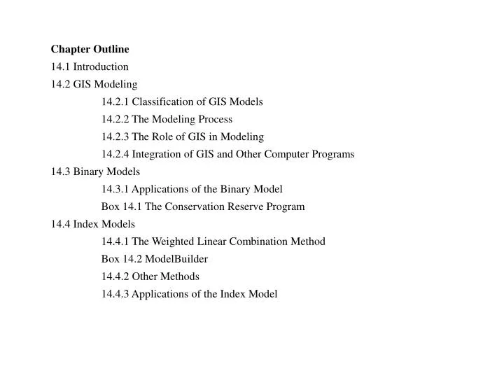
Chapter Outline 14.1 Introduction 14.2 GIS Modeling 14.2.1 Classification of GIS Models 14.2.2 The Modeling Process 14.2.3 The Role of GIS in Modeling 14.2.4 Integration of GIS and Other Computer Programs 14.3 Binary Models 14.3.1 Applications of the Binary Model

E N D
Chapter Outline 14.1 Introduction 14.2 GIS Modeling 14.2.1 Classification of GIS Models 14.2.2 The Modeling Process 14.2.3 The Role of GIS in Modeling 14.2.4 Integration of GIS and Other Computer Programs 14.3 Binary Models 14.3.1 Applications of the Binary Model Box 14.1 The Conservation Reserve Program 14.4 Index Models 14.4.1 The Weighted Linear Combination Method Box 14.2 ModelBuilder 14.4.2 Other Methods 14.4.3 Applications of the Index Model
14.5 Regression Models 14.5.1 Linear Regression Models 14.5.2 Logistic Regression Models 14.6 Process Models 14.6.1 Soil Erosion Models Box 14.3 Explanation of the Six Factors in RUSLE 14.6.2 Other Examples of Process Models 14.6.3 GIS and Process Models
Applications: GIS Modeling Task 1: Build a Vector-based Binary Model Task 2: Build a Raster-based Binary Model Task 3: Build a Vector-based Index Model Task 4: Build a Raster-based Index Model
Suit ID 1 1 3 2 1 2 3 2 3 + + ID Type 2 21 1 1 2 18 3 3 6 Type ID Suit The diagram illustrates a vector-based binary model. First, overlay the two maps so that their spatial features and their attributes (Suit and Type) are combined. Then, use the query statement, Suit = 2 AND Type = 18, to select polygon 4 and save it to the output. 1 3 21 2 3 18 18 1 3 2 1 3 4 2 18 4 2 21 5 7 5 6 6 2 6 6 7 1 Suit = 2 AND Type = 18 4
This diagram illustrates a raster-based binary model. Use the query statement, [Grid1] = 3 AND [Grid2] = 3, to select three cells (shaded) and save then to the output grid.
To build an index model with the selection criteria of slope, aspect, and elevation, the weighted linear combination method involves evaluation at three levels. The first level of evaluation determines the criterion weights (e.g., Ws for slope). The second level of evaluation determines standardized values for each criterion (e.g., s1, s2, and s3 for slope). The third level of evaluation determines the index (aggregate) value for each unit area.
Suit ID S_V 1 1 3 1.0 2 1 0.2 2 3 2 3 0.52 + + ID Type T_V This diagram illustrates a vector-based index model. First, standardize the Suit and Type values of the two input maps into a scale of 0.0 to 1.0. Second, overlay the two maps. Third, assign a weight of 0.4 to the map with Suit and a weight of 0.6 to the map with Type. Finally, calculate the index values for each polygon in the output by summing the weighted criterion values. For example, Polygon 4 has an index value of 0.26 (0.5 *0.4+ 0.1*0.6). 2 21 0.4 1 1 2 18 0.1 3 3 0.83 6 S_V T_V ID 1 0.4 1.0 0.1 2 1.0 3 0.1 0.2 2 1 3 4 0.1 0.5 4 5 0.4 0.5 7 5 6 6 0.8 0.5 7 0.2 0.8 0.46 0.64 0.14 (S_V * 0.4) + (T_V * 0.6) 0.26 0.56 0.44 0.68
This diagram illustrates a raster-based index model. First, standardize the cell values of each input grid into a scale of 0.0 to 1.0. Second, multiply each input grid by its criterion weight. Finally, calculate the index values in the output grid by summing the weighted cell values. For example, the index value of 0.28 is calculated by: 0.12 + 0.04 + 0.12, or 0.2*0.6 + 0.2*0.2 + 0.6*0.2.
Conservation Reserve Program (CRP), Farm Service Agency (FSA) of the U.S. Department of Agriculture http://www.fsa.usda.gov/dafp/cepd/crp.htm California LESA model http://www.consrv.ca.gov/DLRP/qh_lesa.htm WEPP (Water Erosion Prediction Project) http://topsoil.nserl.purdue.edu/nserlweb/weppmain/wepp.html SWAT http://waterhome.tamu.edu/NRCSdata/SWAT_SSURGO Better Assessment Science Integrating point and Nonpoint Sources (BASINS) system http://www.epa.gov/waterscience/BASINS/