Download
1 / 25
250 likes | 354 Vues
Introduction to Statistics − Day 2. Lecture 1 Probability Random variables, probability densities, etc. Brief catalogue of probability densities Lecture 2 The Monte Carlo method Statistical tests Fisher discriminants, neural networks, etc. Lecture 3 Goodness-of-fit tests

E N D
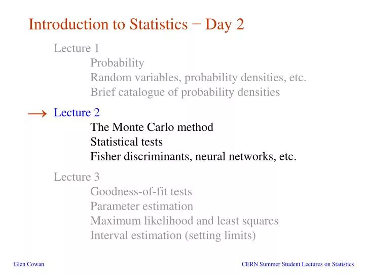
Introduction to Statistics − Day 2 Lecture 1 Probability Random variables, probability densities, etc. Brief catalogue of probability densities Lecture 2 The Monte Carlo method Statistical tests Fisher discriminants, neural networks, etc. Lecture 3 Goodness-of-fit tests Parameter estimation Maximum likelihood and least squares Interval estimation (setting limits) → Glen Cowan CERN Summer Student Lectures on Statistics
The Monte Carlo method What it is: a numerical technique for calculating probabilities and related quantities using sequences of random numbers. The usual steps: (1) Generate sequence r1, r2, ..., rm uniform in [0, 1]. (2) Use this to produce another sequence x1, x2, ..., xn distributed according to some pdf f (x) in which we’re interested (x can be a vector). (3) Use the x values to estimate some property of f (x), e.g., fraction of x values with a < x < b gives → MC calculation = integration (at least formally) MC generated values = ‘simulated data’ →use for testing statistical procedures Glen Cowan CERN Summer Student Lectures on Statistics
Random number generators Goal: generate uniformly distributed values in [0, 1]. Toss coin for e.g. 32 bit number... (too tiring). → ‘random number generator’ = computer algorithm to generate r1, r2, ..., rn. Example: multiplicative linear congruential generator (MLCG) ni+1 = (a ni) mod m , where ni = integer a = multiplier m = modulus n0 = seed (initial value) N.B. mod = modulus (remainder), e.g. 27 mod 5 = 2. This rule produces a sequence of numbers n0, n1, ... Glen Cowan CERN Summer Student Lectures on Statistics
Random number generators (2) The sequence is (unfortunately) periodic! Example (see Brandt Ch 4): a = 3, m = 7, n0 = 1 ← sequence repeats Choose a, m to obtain long period (maximum = m- 1); m usually close to the largest integer that can represented in the computer. Only use a subset of a single period of the sequence. Glen Cowan CERN Summer Student Lectures on Statistics
Random number generators (3) are in [0, 1] but are they ‘random’? Choose a, m so that the ri pass various tests of randomness: uniform distribution in [0, 1], all values independent (no correlations between pairs), e.g. L’Ecuyer, Commun. ACM 31 (1988) 742 suggests a = 40692 m = 2147483399 Far better algorithms available, e.g. RANMAR, period See F. James, Comp. Phys. Comm. 60 (1990) 111; Brandt Ch. 4 Glen Cowan CERN Summer Student Lectures on Statistics
The transformation method Given r1, r2,..., rn uniform in [0, 1], find x1, x2,..., xn that follow f (x) by finding a suitable transformation x (r). Require: i.e. That is, set and solve for x (r). Glen Cowan CERN Summer Student Lectures on Statistics
Example of the transformation method Exponential pdf: Set and solve for x (r). works too.) → Glen Cowan CERN Summer Student Lectures on Statistics
The acceptance-rejection method Enclose the pdf in a box: (1)Generate a random number x, uniform in [xmin, xmax], i.e. r1 is uniform in [0,1]. (2)Generate a 2nd independent random number u uniformly distributed between 0 and fmax, i.e. (3)If u < f (x), then accept x. If not, reject x and repeat. Glen Cowan CERN Summer Student Lectures on Statistics
Example with acceptance-rejection method If dot below curve, use x value in histogram. Glen Cowan CERN Summer Student Lectures on Statistics
Monte Carlo event generators Simple example: e+e-→ m+m- Generate cosq and f: Less simple: ‘event generators’ for a variety of reactions: e+e- → m+m-, hadrons, ... pp → hadrons, D-Y, SUSY,... e.g. PYTHIA, HERWIG, ISAJET... Output = ‘events’, i.e., for each event we get a list of generated particles and their momentum vectors, types, etc. Glen Cowan CERN Summer Student Lectures on Statistics
Monte Carlo detector simulation Takes as input the particle list and momenta from generator. Simulates detector response: multiple Coulomb scattering (generate scattering angle), particle decays (generate lifetime), ionization energy loss (generate D), electromagnetic, hadronic showers, production of signals, electronics response, ... Output = simulated raw data → input to reconstruction software: track finding, fitting, etc. Predict what you should see at ‘detector level’ given a certain hypothesis for ‘generator level’. Compare with the real data. Estimate ‘efficiencies’ = #events found / # events generated. Programming package: GEANT Glen Cowan CERN Summer Student Lectures on Statistics
Statistical tests (in a particle physics context) Suppose the result of a measurement for an individual event is a collection of numbers x1 = number of muons, x2 = mean pt of jets, x3 = missing energy, ... follows some n-dimensional joint pdf, which depends on the type of event produced, i.e., was it For each reaction we consider we will have a hypothesis for the pdf of , e.g., etc. Often call H0 the signal hypothesis (the event type we want); H1, H2, ... are background hypotheses. Glen Cowan CERN Summer Student Lectures on Statistics etc.
Selecting events Suppose we have a data sample with two kinds of events, corresponding to hypotheses H0 and H1 and we want to select those of type H0. Each event is a point in space. What ‘decision boundary’ should we use to accept/reject events as belonging to event type H0? H1 Perhaps select events with ‘cuts’: H0 accept Glen Cowan CERN Summer Student Lectures on Statistics
Other ways to select events Or maybe use some other sort of decision boundary: linear or nonlinear H1 H1 H0 H0 accept accept How can we do this in an ‘optimal’ way? What are the difficulties in a high-dimensional space? Glen Cowan CERN Summer Student Lectures on Statistics
Test statistics Construct a ‘test statistic’ of lower dimension (e.g. scalar) Try to compactify data without losing ability to discriminate between hypotheses. We can work out the pdfs Decision boundary is now a single ‘cut’ on t. This effectively divides the sample space into two regions, where we accept or reject H0. Glen Cowan CERN Summer Student Lectures on Statistics
Significance level and power of a test Probability to reject H0 if it is true (error of the 1st kind): (significance level) Probability to accept H0 if H1 is true (error of the 2nd kind): (1 - b = power) Glen Cowan CERN Summer Student Lectures on Statistics
Efficiency of event selection Probability to accept an event which is signal (signal efficiency): Probability to accept an event which is background (background efficiency): Glen Cowan CERN Summer Student Lectures on Statistics
Purity of event selection Suppose only one background type b; overall fractions of signal and background events are ps and pb (prior probabilities). Suppose we select events with t < tcut. What is the ‘purity’ of our selected sample? Here purity means the probability to be signal given that the event was accepted. Using Bayes’ theorem we find: So the purity depends on the prior probabilities as well as on the signal and background efficiencies. Glen Cowan CERN Summer Student Lectures on Statistics
Constructing a test statistic How can we select events in an ‘optimal way’? Neyman-Pearson lemma (proof in Brandt Ch. 8) states: To get the lowest eb for a given es (highest power for a given significance level), choose acceptance region such that where c is a constant which determines es. Equivalently, optimal scalar test statistic is Glen Cowan CERN Summer Student Lectures on Statistics
Why Neyman-Pearson doesn’t always help The problem is that we usually don’t have explicit formulae for the pdfs Instead we may have Monte Carlo models for signal and background processes, so we can produce simulated data, and enter each event into an n-dimensional histogram. Use e.g. M bins for each of the n dimensions, total of Mn cells. But n is potentially large, →prohibitively large number of cells to populate with Monte Carlo data. Compromise: make Ansatz for form of test statistic with fewer parameters; determine them (e.g. using MC) to give best discrimination between signal and background. Glen Cowan CERN Summer Student Lectures on Statistics
Linear test statistic Ansatz: Choose the parameters a1, ..., an so that the pdfs have maximum ‘separation’. We want: ms g (t) mb large distance between mean values, small widths ss sb t → Fisher: maximize Glen Cowan CERN Summer Student Lectures on Statistics
Fisher discriminant Using this definition of separation gives a Fisher discriminant. H1 Corresponds to a linear decision boundary. H0 accept Equivalent to Neyman-Pearson if the signal and background pdfs are multivariate Gaussian with equal covariances; otherwise not optimal, but still often a simple, practical solution. Glen Cowan CERN Summer Student Lectures on Statistics
Nonlinear test statistics The optimal decision boundary may not be a hyperplane, →nonlinear test statistic H1 Multivariate statistical methods are a Big Industry: Neural Networks, Support Vector Machines, Kernel density methods, ... H0 accept Particle Physics can benefit from progress in Machine Learning. Glen Cowan CERN Summer Student Lectures on Statistics
Neural network example from LEP II Signal: e+e-→ W+W- (often 4 well separated hadron jets) Background: e+e-→ qqgg (4 less well separated hadron jets) ← input variables based on jet structure, event shape, ... none by itself gives much separation. Neural network output does better... (Garrido, Juste and Martinez, ALEPH 96-144) Glen Cowan CERN Summer Student Lectures on Statistics
Wrapping up lecture 2 We’ve seen the Monte Carlo method: calculations based on sequences of random numbers, used to simulate particle collisions, detector response. And we looked at statistical tests and related issues: discriminate between event types (hypotheses), determine selection efficiency, sample purity, etc. Some modern (and less modern) methods were mentioned: Fisher discriminants, neural networks, support vector machines,... In the next lecture we will talk about goodness-of-fit tests and then move on to another main subfield of statistical inference:parameter estimation. Glen Cowan CERN Summer Student Lectures on Statistics