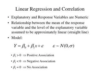
Linear Regression and Correlation Analysis

Regression Analysis Regression Analysis attempts to determine the strength of the relationship between one dependent variable (usually denoted by Y) and a series of other changing variables (known as independent variables).

Regression Analysis Regression Analysis is used to: Predict the value of a dependent variable based on the value of at least one independent variable Explain the impact of changes in an independent variable on the dependent variable Dependent Variable: The variable we wish to explain Independent Variable: The variable used to explain the dependent variable

Regression Analysis One of the two variables (X, Y), say X is an independent variable/ controlled variable/ ordinary variable, Y is random Variable Relationship between X and Y is described by a linear function Dependence of Y on X or Regression of Y on X Dependence of Blood Pressure Y on X Regression of gain of weight Y on food X

Types of Regression Models Positive Linear Relationship Relationship NOT Linear Negative Linear Relationship No Relationship

Regression Analysis In Regression Analysis the dependence of Y on x is the dependence of mean µ of Y on x µ = µ (x) The curve of µ (x) is called Regression Curve Straight Regression Line is: µ (x) = k0 + k1 x

Estimated Regression Model The sample regression line provides an estimate of the population regression line Estimated (or predicted) value Estimate of the Regression Intercept Estimate of the Regression Slope Independent Variable

Least Squares Principle The straight Line should be fitted through the given points, so that the sum of squares of distances of those points from the line is minimum, where the distance is measured in Vertical Direction. The x-values x1, x2,…, xnin the Sample (x1, y1), (x2, y2), …, (xn, yn) are not all equal.

Sample Regression Line (Regression Coefficient)

Sample Regression Line Sxy= Sample Covariance Sx2 = Variance of X values Sy2 = Variance of Y values

Sample Regression Line The decrease of values y[%] of Leather for certain fixed values of High Pressure X[atmosphere] was measured. Find Regression Line of Y on X.

Sample Regression Line (Regression Coefficient)

Sample Regression Line Regression Line = y = 0.0077x - 0.64

Formula: Regression Line Intercept Slope of the Line

Equation of Regression Line

Problem 1 Find and sketch or graph the Sample Regression Line of y and x for the points (-1, 1), (0, 1.7), and (1, 3).

Problem 3 Find and sketch or graph the Sample Regression Line of y and x for the points (2, 12), (5, 24), (9, 33) and (14, 50).

Problem 5 Find and sketch or graph the Sample Regression Line of y and x for the given data: Also find Stopping Distance at 35 mph.

Problem 7 Find and sketch or graph the Sample Regression Line of y and x for the given data:

Problem 9 Find and sketch or graph the Sample Regression Line of y and x for the given data:

Confidence IntervalAssumptions The x-values x1, x2,…, xnin the Sample (x1, y1), (x2, y2), …, (xn, yn) are not all equal. For each fixed x, the random variable Y is normal with mean µ (x) = k0 + k1 x and variance б2 independent of x The n performances of the experiment by which we obtain a sample (x1, y1), (x2, y2), …, (xn, yn) are independent.

Steps to FindConfidence Interval Choose a Confidence Level γ (95%, 99%, etc) Determine the solution C of the equation F(C) = ½ (1 + γ) [ Table t-distribution with n-2 df ] Using Sample Compute (n-1)Sx2, (n-1)Sxy and K1 Compute K Confidence Interval (K1 – K ≤ K1 ≤ K1 + K)

Problem 11 Find a 95% Confidence Interval for the Regression Coefficient K1, Assuming that A2 and A3 hold, for the given Sample data:

Correlation Analysis Both variables (X, Y) are random variables Grades X and Y of students in Math and Physics Hardness X of steel plates in the centre and hardness Y near the edges of the plates

Scatter Plots and Correlation A scatter plot (or scatter diagram) is used to show the relationship between two variables Correlation analysis is used to measure strength of the association (linear relationship) between two variables Only concerned with strength of the relationship No causal effect is implied

Scatter Plot Examples Linear relationships Curvilinear relationships y y x x y y x x

Scatter Plot Examples Strong relationships Weak relationships y y x x y y x x

Correlation Coefficient The population correlation coefficient ρ(rho) measures the strength of the association between the variables The sample correlation coefficient r is an estimate of ρ and is used to measure the strength of the linear relationship in the sample observations

Features of ρand r Unit free Range between -1 and 1 The closer to -1, the stronger the negative linear relationship The closer to 1, the stronger the positive linear relationship The closer to 0, the weaker the linear relationship

Approximate r Values y y y x x x r = -1 r = -.6 r = 0 y y x x r = +.3 r = +1

Population Correlation Coefficient Theorem: The Correlation Coefficient ρ satisfies -1 ≤ ρ ≤ 1. In particular ρ = ±1, if and only if X and Y are linearly related i.e Y = rX + δ X = r*Y + δ* X and Y are called uncorrelated, if ρ = 0.

Theorem (Normal Distribution) Independent X and Y are uncorrelated. If (X, Y) is normal, the uncorrelated X and Y are independent. Example: If X assumes -1, 0, 1 with probability 1/3. and Y = X2

Test ForCorrelation Coefficient : ρ Test H0: ρ = 0 and H1: ρ > 0 Choose a Significance Level α (5%, 1%, etc) Determine the solution C of the equation P(T ≤ C) = 1 - α [ Table t-distribution with n-2 df ] Compute r and t If t ≤ C, accept the Hypothesis, otherwise reject the Hypothesis.

Example:Correlation Coefficient

Calculation Example Tree Height, y r = 0.886 → relatively strong positive linear association between x and y Trunk Diameter, x

Excel Output Excel Correlation Output Tools / data analysis / correlation… Correlation between Tree Height and Trunk Diameter

Significance Test for Correlation Hypotheses H0: ρ = 0 (no correlation) HA: ρ≠ 0 (correlation exists) Test statistic (with n – 2 degrees of freedom)

Example: Produce Stores Is there evidence of a linear relationship between tree height and trunk diameter at the .05 level of significance? H0: ρ= 0 (No correlation) H1: ρ≠ 0 (correlation exists) =.05 , df=8 - 2 = 6

Example: Test Solution Decision:Reject H0 Conclusion:There is evidence of a linear relationship at the 5% level of significance d.f. = 8-2 = 6 a/2=.025 a/2=.025 Reject H0 Do not reject H0 Reject H0 -tα/2 tα/2 0 -2.4469 2.4469 4.68

Population Linear Regression The population regression model: Random Error term, or residual Population SlopeCoefficient Population y intercept Independent Variable Dependent Variable Linear component Random Error component

Linear Regression Assumptions Error values (ε) are statistically independent Error values are normally distributed for any given value of x The probability distribution of the errors is normal The probability distribution of the errors has constant variance The underlying relationship between the x variable and the y variable is linear

Population Linear Regression (continued) y Observed Value of y for xi εi Slope = β1 Predicted Value of y for xi Random Error for this x value Intercept = β0 x xi

Residual Analysis Purposes Examine for linearity assumption Examine for constant variance for all levels of x Evaluate normal distribution assumption Graphical Analysis of Residuals Can plot residuals vs. x Can create histogram of residuals to check for normality

Residual Analysis for Linearity y y x x x x residuals residuals  Not Linear Linear

Residual Analysis for Constant Variance y y x x x x residuals residuals  Constant variance Non-constant variance

Excel Output

Simple Linear Regression Example A real estate agent wishes to examine the relationship between the selling price of a home and its size (measured in square feet) A random sample of 10 houses is selected Dependent variable (y) = house price in $1000s Independent variable (x) = square feet

Sample Data for House Price Model

Regression Using Excel

Excel Output The regression equation is:

Graphical Presentation House price model: scatter plot and regression line Slope = 0.10977 Intercept = 98.248

Interpretation of the Intercept, b0 b0 is the estimated average value of Y when the value of X is zero (if x = 0 is in the range of observed x values) Here, no houses had 0 square feet, so b0 = 98.24833 just indicates that, for houses within the range of sizes observed, $98,248.33 is the portion of the house price not explained by square feet

Interpretation of the Slope Coefficient, b1 b1 measures the estimated change in the average value of Y as a result of a one-unit change in X Here, b1 = .10977 tells us that the average value of a house increases by .10977($1000) = $109.77, on average, for each additional one square foot of size

Least Squares Regression Properties The sum of the residuals from the least squares regression line is 0 ( ) The sum of the squared residuals is a minimum (minimized ) The simple regression line always passes through the mean of the y variable and the mean of the x variable The least squares coefficients are unbiased estimates of β0 and β1

Explained and Unexplained Variation Total variation is made up of two parts: Total sum of Squares Sum of Squares Error Sum of Squares Regression where: = Average value of the dependent variable y = Observed values of the dependent variable = Estimated value of y for the given x value

Explained and Unexplained Variation SST = total sum of squares Measures the variation of the yi values around their mean y SSE = error sum of squares Variation attributable to factors other than the relationship between x and y SSR = regression sum of squares Explained variation attributable to the relationship between x and y

Explained and Unexplained Variation y yi   y SSE= (yi-yi )2 _ SST=(yi-y)2  _ y  SSR = (yi -y)2 _ _ y y x Xi

Coefficient of Determination, R2 The coefficient of determination is the portion of the total variation in the dependent variable that is explained by variation in the independent variable The coefficient of determination is also called R-squared and is denoted as R2 where

Coefficient of Determination, R2 Coefficient of determination Note: In the single independent variable case, the coefficient of determination is where: R2 = Coefficient of determination r = Simple correlation coefficient

Examples of Approximate R2 Values y R2 = 1 Perfect linear relationship between x and y: 100% of the variation in y is explained by variation in x x R2 = 1 y x R2 = +1

Examples of Approximate R2 Values y 0 < R2 < 1 Weaker linear relationship between x and y: Some but not all of the variation in y is explained by variation in x x y x

Examples of Approximate R2 Values R2 = 0 y No linear relationship between x and y: The value of Y does not depend on x. (None of the variation in y is explained by variation in x) x R2 = 0

Excel Output 58.08% of the variation in house prices is explained by variation in square feet

Standard Error of Estimate The standard deviation of the variation of observations around the regression line is estimated by Where SSE = Sum of squares error n = Sample size k = number of independent variables in the model

The Standard Deviation of the Regression Slope The standard error of the regression slope coefficient (b1) is estimated by where: = Estimate of the standard error of the least squares slope = Sample standard error of the estimate

Excel Output

Comparing Standard Errors Variation of observed y values from the regression line Variation in the slope of regression lines from different possible samples y y x x y y x x

Inference about the Slope: t Test t test for a population slope Is there a linear relationship between x and y? Null and alternative hypotheses H0: β1 = 0 (no linear relationship) H1: β1 0 (linear relationship does exist) Test statistic where: b1 = Sample regression slope coefficient β1 = Hypothesized slope sb1 = Estimator of the standard error of the slope

Inference about the Slope: t Test (continued) Estimated Regression Equation: The slope of this model is 0.1098 Does square footage of the house affect its sales price?

H0: β1 = 0 HA: β1 0 Inferences about the Slope: tTest Example Test Statistic: t = 3.329 b1 t From Excel output: d.f. = 10-2 = 8 Decision: Conclusion: Reject H0 a/2=.025 a/2=.025 There is sufficient evidence that square footage affects house price Reject H0 Do not reject H0 Reject H0 -tα/2 tα/2 0 -2.3060 2.3060 3.329

Regression Analysis for Description Confidence Interval Estimate of the Slope: d.f. = n - 2 Excel Printout for House Prices: At 95% level of confidence, the confidence interval for the slope is (0.0337, 0.1858)

Regression Analysis for Description Since the units of the house price variable is $1000s, we are 95% confident that the average impact on sales price is between $33.70 and $185.80 per square foot of house size This 95% confidence interval does not include 0. Conclusion: There is a significant relationship between house price and square feet at the .05 level of significance

Confidence Interval for the Average y, Given x Confidence interval estimate for the mean of y given a particular xp Size of interval varies according to distance away from mean, x

Confidence Interval for an Individual y, Given x Confidence interval estimate for an Individual value of y given a particular xp This extra term adds to the interval width to reflect the added uncertainty for an individual case

Interval Estimates for Different Values of x Prediction Interval for an individual y, given xp y Confidence Interval for the mean of y, given xp  y = b0 + b1x x xp x

Example: House Prices Estimated Regression Equation: Predict the price for a house with 2000 square feet

Example: House Prices (continued) Predict the price for a house with 2000 square feet: The predicted price for a house with 2000 square feet is 317.85($1,000s) = $317,850

Estimation of Mean Values: Example Confidence Interval Estimate for E(y)|xp Find the 95% confidence interval for the average price of 2,000 square-foot houses  Predicted Price Yi = 317.85 ($1,000s) The confidence interval endpoints are 280.66 -- 354.90, or from $280,660 -- $354,900

Estimation of Individual Values: Example Prediction Interval Estimate for y|xp Find the 95% confidence interval for an individual house with 2,000 square feet  Predicted Price Yi = 317.85 ($1,000s) The prediction interval endpoints are 215.50 -- 420.07, or from $215,500 -- $420,070

Linear Regression and Correlation Analysis