Download
1 / 29
290 likes | 437 Vues
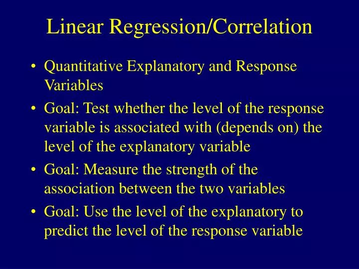
Linear Regression/Correlation. Quantitative Explanatory and Response Variables Goal: Test whether the level of the response variable is associated with (depends on) the level of the explanatory variable Goal: Measure the strength of the association between the two variables

E N D
Linear Regression/Correlation • Quantitative Explanatory and Response Variables • Goal: Test whether the level of the response variable is associated with (depends on) the level of the explanatory variable • Goal: Measure the strength of the association between the two variables • Goal: Use the level of the explanatory to predict the level of the response variable
Linear Relationships • Notation: • Y: Response (dependent, outcome) variable • X: Explanatory (independent, predictor) variable • Linear Function (Straight-Line Relation): • Y = a + b X (Plot Y on vertical axis, X horizontal) • Slope (b): The amount Y changes when X increases by 1 • b > 0 Line slopes upward (Positive Relation) • b = 0 Line is flat (No linear Relation) • b < 0 Line slopes downward (Negative Relation) • Y-intercept (a): Y level when X=0
Example: Service Pricing • Internet History Resources (New South Wales Family History Document Service) • Membership fee: $20A • 20¢ ($0.20A) per image viewed • Y = Total cost of service • X = Number of images viewed • a = Cost when no images viewed • b = Incremental Cost per image viewed • Y = a + b X = 20+0.20X
Probabilistic Models • In practice, the relationship between Y and X is not “perfect”. Other sources of variation exist. We decompose Y into 2 components: • Systematic Relationship with X: a + bX • Random Error: e • Random respones can be written as the sum of the systematic (also thought of as the mean) and random components: Y = a + bX + e • The (conditional on X) mean response is: • E(Y) = a + bX
Least Squares Estimation • Problem: a, b are unknown parameters, and must be estimated and tested based on sample data. • Procedure: • Sample n individuals, observing X and Y on each one • Plot the pairs Y (vertical axis) versus X (horizontal) • Choose the line that “best fits” the data. • Criteria: Choose line that minimizes sum of squared vertical distances from observed data points to line. Least Squares Prediction Equation:
Example - Pharmacodynamics of LSD • Response (Y) - Math score (mean among 5 volunteers) • Predictor (X) - LSD tissue concentration (mean of 5 volunteers) • Raw Data and scatterplot of Score vs LSD concentration: Source: Wagner, et al (1968)
Example - Pharmacodynamics of LSD (Column totals given in bottom row of table)
Example - Retail Sales • U.S. SMSA’s • Y = Per Capita Retail Sales • X = Females per 100 Males
Residuals • Residuals (aka Errors): Difference between observed values and predicted values: • Error sum of squares: • Estimate of (conditional) standard deviation of Y:
Linear Regression Model • Data: Y = a + b X + e • Mean: E(Y) = a + b X • Conditional Standard Deviation: s • Error terms (e) are assumed to be independent and normally distributed
Correlation Coefficient • Slope of the regression describes the direction of association (if any) between the explanatory (X) and response (Y). Problems: • The magnitude of the slope depends on the units of the variables • The slope is unbounded, doesn’t measure strength of association • Some situations arise where interest is in association between variables, but no clear definition of X and Y • Population Correlation Coefficient: r • Sample Correlation Coefficient: r
Correlation Coefficient • Pearson Correlation: Measure of strength of linear association: • Does not delineate between explanatory and response variables • Is invariant to linear transformations of Y and X • Is bounded between -1 and 1 (higher values in absolute value imply stronger relation) • Same sign (positive/negative) as slope
Example - Pharmacodynamics of LSD • Using formulas for standard deviation from beginning of course: sX = 1.935 and sY = 18.611 • From previous calculations: b = -9.01 This represents a strong negative association between math scores and LSD tissue concentration
Coefficient of Determination • Measure of the variation in Y that is “explained” by X • Step 1: Ignoring X, measure the total variation in Y (around its mean): • Step 2: Fit regression relating Y to X and measure the unexplained variation in Y (around its predicted values): • Step 3: Take the difference (variation in Y “explained” by X), and divide by total:
Inference Concerning the Slope (b) • Parameter: Slope in the population model(b) • Estimator: Least squares estimate: b • Estimated standard error: • Methods of making inference regarding population: • Hypothesis tests (2-sided or 1-sided) • Confidence Intervals
2-Sided Test H0: b = 0 HA: b 0 1-sided Test H0: b = 0 HA+: b> 0 or HA-: b< 0 Significance Test for b
(1-a)100% Confidence Interval for b • Conclude positive association if entire interval above 0 • Conclude negative association if entire interval below 0 • Cannot conclude an association if interval contains 0 • Conclusion based on interval is same as 2-sided hypothesis test
Example - Pharmacodynamics of LSD • Testing H0: b = 0 vs HA: b 0 • 95% Confidence Interval for b : t.025,5
Analysis of Variance in Regression • Goal: Partition the total variation in y into variation “explained” by x and random variation • These three sums of squares and degrees of freedom are: • Total (TSS) dfTotal = n-1 • Error (SSE) dfError = n-2 • Model (SSR) dfModel = 1
Analysis of Variance in Regression • Analysis of Variance - F-test • H0: b = 0 HA: b 0 F represents the F-distribution with 1 numerator and n-2 denominator degrees of freedom
Example - Pharmacodynamics of LSD • Total Sum of squares: • Error Sum of squares: • Model Sum of Squares:
Example - Pharmacodynamics of LSD • Analysis of Variance - F-test • H0: b = 0 HA: b 0
Significance Test for Pearson Correlation • Test identical (mathematically) to t-test for b, but more appropriate when no clear explanatory and response variable • H0: r = 0 Ha: r 0 (Can do 1-sided test) • Test Statistic: • P-value: 2P(t|tobs|)
Model Assumptions & Problems • Linearity: Many relations are not perfectly linear, but can be well approximated by straight line over a range of X values • Extrapolation: While we can check validity of straight line relation within observed X levels, we cannot assume relationship continues outside this range • Influential Observations: Some data points (particularly ones with extreme X levels) can exert a large influence on the predicted equation.