Download
1 / 45
460 likes | 586 Vues
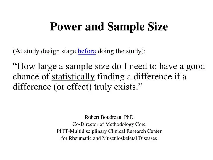
Power and Sample Size (At study design stage before doing the study): “How large a sample size do I need to have a good chance of statistically finding a difference if a difference (or effect) truly exists.” Robert Boudreau, PhD Co-Director of Methodology Core

E N D
Power and Sample Size (At study design stage before doing the study): “How large a sample size do I need to have a good chance of statistically finding a difference if a difference (or effect) truly exists.” Robert Boudreau, PhD Co-Director of Methodology Core PITT-Multidisciplinary Clinical Research Center for Rheumatic and Musculoskeletal Diseases
PHARYNX • A Clinical Trial in the Treatment of Carcinoma of the Oropharynx • SIZE: 195 observations SEX Frequency Percent Male 149 76.4 Female 46 23.6 Standard treatment:Radiation therapy alone (n=100) Test treatment: Radiation + Chemotherapy (n=95)
Post Treatment: 1 Yr Mortality Signif Diffs By Gender (?) % died < 1 yr ‚Standard‚ Test ‚P-value‚ ƒƒƒƒƒƒƒƒƒˆƒƒƒƒƒƒƒƒˆƒƒƒƒƒƒƒƒˆƒƒƒƒƒƒƒˆ Men ‚ 42.1% ‚ 45.7% ‚ 0.66 ‚ ‚ ‚ ‚ ‚ (n=146) ‚ (32/76)‚ (32/70)‚ ‚ ƒƒƒƒƒƒƒƒƒˆƒƒƒƒƒƒƒƒˆƒƒƒƒƒƒƒƒˆƒƒƒƒƒƒƒˆ Women ‚ 21.7% ‚ 52.2% ‚ 0.03 ‚ ‚ ‚ ‚ ‚ (n=46) ‚ (5/23) ‚ (12/23)‚ ‚ ƒƒƒƒƒƒƒƒƒˆƒƒƒƒƒƒƒƒˆƒƒƒƒƒƒƒƒˆƒƒƒƒƒƒƒˆ Frequency Missing = 3 (censored before 1yr) • Large difference in women detected (even with smaller N)
Is Stage of Cancer a Factor ? T_STAGE • 1=primary tumor measuring 2 cm or less in largest diameter, • 2=primary tumor measuring 2 cm to 4 cm in largest diameter with minimal infiltration in depth • 3=primary tumor measuring more than 4 cm, 4=massive invasive tumor N_STAGE (see Cooper et. al, NEJM: Stage 2+ => high mortality) • 0=no clinical evidence of node metastases • 1=single positive node 3 cm or less in diameter, not fixed • 2=single positive node more than 3 cm in diameter, not fixed • 3=multiple positive nodes or fixed positive nodes
Is Stage of Cancer a Factor ? Cooper JS, et.al. Postoperative Concurrent Radiotherapy and Chemotherapy for High-Risk Squamous-Cell Carcinoma of the Head and Neck. NEJM 350(19):1937-1944. May 6, 2004 • “Patients who have two or more regional lymph nodes involved, extracapsular spread of disease, or microscopically involved mucosal margins of resection have particularly high rates of local recurrence (27 to 61 percent) and distant metastases (18 to 21 percent) and a high risk of death (five-year survival rate, 27 to 34 percent).”
Males: Tumor Stage by Metastasized Nodes -------------------------------- SEX=Male ----------------------- The FREQ Procedure Table of T_STAGE by N_STAGE T_STAGE(T_STAGE) N_STAGE(N_STAGE) Frequency‚ 0 ‚ 1 ‚ 2 ‚ 3 ‚ Total ƒƒƒƒƒƒƒƒƒˆƒƒƒƒƒƒƒƒˆƒƒƒƒƒƒƒƒˆƒƒƒƒƒƒƒƒˆƒƒƒƒƒƒƒƒˆ 1 ‚ 0 ‚ 0 ‚ 3 ‚ 5 ‚ 8 ƒƒƒƒƒƒƒƒƒˆƒƒƒƒƒƒƒƒˆƒƒƒƒƒƒƒƒˆƒƒƒƒƒƒƒƒˆƒƒƒƒƒƒƒƒˆ 2 ‚ 0 ‚ 0 ‚ 9 ‚ 10 ‚ 19 ƒƒƒƒƒƒƒƒƒˆƒƒƒƒƒƒƒƒˆƒƒƒƒƒƒƒƒˆƒƒƒƒƒƒƒƒˆƒƒƒƒƒƒƒƒˆ 3 ‚ 17 ‚ 11 ‚ 11 ‚ 29 ‚ 68 ƒƒƒƒƒƒƒƒƒˆƒƒƒƒƒƒƒƒˆƒƒƒƒƒƒƒƒˆƒƒƒƒƒƒƒƒˆƒƒƒƒƒƒƒƒˆ 4 ‚ 13 ‚ 9 ‚ 2 ‚ 30 ‚ 54 ƒƒƒƒƒƒƒƒƒˆƒƒƒƒƒƒƒƒˆƒƒƒƒƒƒƒƒˆƒƒƒƒƒƒƒƒˆƒƒƒƒƒƒƒƒˆ Total 30 20 25 74 149
Males: 1 Year Mortality(Among those with none or 1 small node) TX(TX) died < 1 yr Frequency‚ Row Pct ‚ 0‚ 1‚ Total ƒƒƒƒƒƒƒƒƒˆƒƒƒƒƒƒƒƒˆƒƒƒƒƒƒƒƒˆ Standard ‚ 20 ‚ 9 ‚ 29 ‚ 68.97 ‚ 31.03 ‚ ƒƒƒƒƒƒƒƒƒˆƒƒƒƒƒƒƒƒˆƒƒƒƒƒƒƒƒˆ Test ‚ 10 ‚ 10 ‚ 20 ‚ 50.00 ‚ 50.00 ‚ ƒƒƒƒƒƒƒƒƒˆƒƒƒƒƒƒƒƒˆƒƒƒƒƒƒƒƒˆ Total 30 19 49 Frequency Missing = 1 Statistics for Table of TX by died_lt_1yr Statistic DF Value Prob ƒƒƒƒƒƒƒƒƒƒƒƒƒƒƒƒƒƒƒƒƒƒƒƒƒƒƒƒƒƒƒƒƒƒƒƒƒƒƒƒƒƒƒƒƒƒƒƒƒƒƒƒƒƒ Chi-Square 1 1.7934 0.1805 • Not quite Statistically Significant
Males: 1 Year Mortality(Among those with none or 1 small node) WHAT IF: Exact same rates, but 5 times as many in study (n=245 vs 49) TX(TX) died < 1 yr Frequency‚ Row Pct ‚ 0‚ 1‚ Total ƒƒƒƒƒƒƒƒƒˆƒƒƒƒƒƒƒƒˆƒƒƒƒƒƒƒƒˆ Standard ‚ 100 ‚ 45 ‚ 145 ‚ 68.97 ‚ 31.03 ‚ ƒƒƒƒƒƒƒƒƒˆƒƒƒƒƒƒƒƒˆƒƒƒƒƒƒƒƒˆ Test ‚ 50 ‚ 50 ‚ 100 ‚ 50.00 ‚ 50.00 ‚ ƒƒƒƒƒƒƒƒƒˆƒƒƒƒƒƒƒƒˆƒƒƒƒƒƒƒƒˆ Total 150 95 245 Frequency Missing = 5 Statistics for Table of TX by died_lt_1yr Statistic DF Value Prob ƒƒƒƒƒƒƒƒƒƒƒƒƒƒƒƒƒƒƒƒƒƒƒƒƒƒƒƒƒƒƒƒƒƒƒƒƒƒƒƒƒƒƒƒƒƒƒƒƒƒƒƒƒƒ Chi-Square 1 8.9670 0.0027
Sampling Variability, Power and Sample Size Standard Treatment Case 1: n=29 (original study sample size) p1= sample estimate of prob of death < 1 yr = 9/29 = 0.3103 Stderr(p1) = sqrt ( p1*(1-p1) / n1 ) = sqrt ( 0.3103*0.6897/29) = 0.0859 (8.6%) Case 2: n=145 (if 5 times larger sample size) p1* = 45/145= 0.3103 Stderr(p1) = sqrt(0.3103*0.6897/ 145) = 0.0384 (3.8%)) = Stderr(p1) / sqrt(5) = Stderr(p1) / 2.236
Sampling Variability, Power and Sample Size (cont’d) Standard Test Difference . n1 p1 Stderr(p1) n2 p2 Stderr(p2) p2-p1 Stderr(p2-p1) Z (ratio) 29 0.3105 0.0859 20 0.50 0.1180 0.1895 0.1460 1.30 • 0.3105 0.0384 100 0.50 0.0500 0.1895 0.0653 2.90 In both cases • The null hypothesis is H0: True Diff=0 • P[ Type I error ] = P[ Reject H0 when H0 true ] = 0.05 Case #1: Observed diff. explainable “by chance” (Z=1.30, p=0.1936) Case #2: Observed diff. not explainable “by chance” (Z=3.01, p=0.0037) “Level of significance”, “alpha-level"
Distribution of possible observed p2-p1 for different sample sizes under hypothetical condition that the mortality rates are really the same n=245 per group n=49 per group
Two-sided Hypothesis Test (2 treatments equal vs not equal ?) n=49, p=0.1936 n=245, p=0.0037 (Pvalue)/2
Sampling Variability, Power and Sample Size (cont’d) • Null Hypothesis: 1 yr mortality rates are same • Alternate Hypothesis: 1 yr mortality rates differ by treatment Natural Question: Is there actually a difference, but the small sample size study didn’t find it ? • Type II Error: Accept null hypothesis when alternate hypothesis is true • Prob[Type II Error] = β • Power = Prob[ Reject Ho when alternate true] = 1 - β
Making Decisions Using Statistical Tests: Type I & Type II Errors
Power & Sample Size Cooper et. al. NEJM • “On the basis of the previous trials of the RTOG, patients treated with postoperative radiation were expected to have a two-year rate of local or regional recurrence of 38 percent. The study required the randomization of 398 eligible patients to have the statistical power to detect an absolute improvement of 15 percent in this rate with the use of a two-sided test with 0.80 statistical power and a significance level of 0.05.
Power & Sample Size Calculations • Power & sample size calculations are typically made using estimated rates from prior or related studies • A scientifically meaningful improvement, change, difference, odds-ratio (OR) or hazard-ratio (HR) is set, then a required sample size to achieve 80% power is computed. • The budget may dictate the maximum available “N”. => Power is then calculated based on fixed “N” for a range of differences, ORs or HRs. Prior studies are used to estimate means, stdevs, rates, ORs … etc.
A. Power with sample size (N) fixed Power = Prob[ finding signif difference if recurrence rates differ by tabulated amounts] * Using two-sample independent chi-square test
A. Power with sample size (N) fixed • Null Hypothesis: 1 yr mortality rates are same • Alternate Hypothesis: 1 yr mortality rates differ by treatment Test statistic: Z = (p1 – p2) / Stderr(p1-p2) Stderr(p1-p2) =sqrt( var(p1-p2) ) =sqrt( p1*(1-p1)/n + p2*(1-p2)/n ) Z is approximately Normal (for any p1, p2) with mean: (p1-p2)/stderr (=0 if no difference) with SD=1 (aka “standarized”)
A. Power with sample size fixed(n=150 each group) Rejection Region ← | | → Rejection Region ←Alt #3: p1=0.38, p2=0.23 (recurrence rates) (radiation) (rad + chemo) Power=0.809 = Prob [ in rejection region ] ←Alt #3: p1=0.38, p2=0.23 (radiation) (rad + chemo) Power=0.809 = Prob [ in rejection region ] ←Null Hypothesis distribution is red
A. Power with sample size (N) fixed Z = (p1 – p2) / stderr Under Alt #3, distribution of Z has mean: (0.38 – 0.23) / 0.052 = 0.15 / 0.052 = 2.86 → 80.9% of area is to right of null hypothesis (no diff) rejection region → Reject H0 if |Z| > 1.96
A. Power with sample size (N) fixed * In SAS: * Compute power with n=150 * per group with alternate p2=0.23; proc power; twosamplefreq test=pchi groupproportions = (0.38, 0.23) npergroup = 150 power= .; run;
A. Power with sample size (N) fixed The POWER Procedure Pearson Chi-square Test for Two Proportions Fixed Scenario Elements Distribution Asymptotic normal Method Normal approximation Group 1 Proportion 0.38 Group 2 Proportion 0.23 Sample Size Per Group 150 Number of Sides 2 Null Proportion Difference 0 Alpha 0.05 Computed Power Power 0.809
B: Sample size (N) to achieve 80% power * How many needed per group for exactly * 80% power ?; proc power; twosamplefreq test=pchi groupproportions = (0.38, 0.23) npergroup = . power= 0.8; run;
B: Sample size (N) to achieve 80% power The POWER Procedure Pearson Chi-square Test for Two Proportions Fixed Scenario Elements Distribution Asymptotic normal Method Normal approximation Group 1 Proportion 0.38 Group 2 Proportion 0.23 Nominal Power 0.8 Number of Sides 2 Null Proportion Difference 0 Alpha 0.05 Computed N Per Group Actual N Per Power Group 0.801 147
B: Sample size (N) to achieve 80% power * 80% Power = Prob[ finding signif difference if recurrence rates differ by tabulated amounts] Using two-sample independent chi-square test
Actual Results of the Cooper Study Using the Sample Sizes Based on Their Power Calculations (P = 0.01) Rates of Local and Regional Control Cooper JS et al. Postoperative Concurrent Radiotherapy and Chemotherapy for High-Risk Squamous-Cell Carcinoma of the Head and Neck. New Eng J Med. 350 (2004) 1937-1944.
B: Sample size (N) to achieve 80% power Sample Size: Two-sample Test of Proportions
B: Sample size (N) to achieve 80% power * How many are needed per group for exactly * 80% power ? (implements the formula); data _null_; p1=0.38; p2=0.23; p=(p1+p2)/2; n=( 1.96*sqrt( 2*p*(1-p) ) + 0.84*sqrt( p1*(1-p1)+ p2*(1-p2) ) )**2 /(p2-p1)**2; put n=; run; n=146.5414874
BARI 10-Year SurvivalStratified by Diabetes Status No Treated Diabetes CABG vs PTCA: p = 0.50 Treated Diabetes CABG vs PTCA: p = 0.012 Years
Logistic Regression: Sample size (N) to achieve 80% power Goal of new study proposal: Test survival for improved method of PTCA BARI: Diabetics vs Non-Diabetics PTCA 10 yrs survival: p1=0.441, p2=0.768 OR= ( p2/(1-p2) ) / (p1/(1-p1)) = 3.31 Approx 20% of eligible patients are diabetic (in general population)
Logistic Regression: Sample size (N) to achieve 80% power *To Detect OR=1.8 with 80% Power; * 20% diabetics (e.g like cohort study); proc power; twosamplefreq test=pchi oddsratio= 1.8 refproportion=0.441 groupweights=(1 4) ntotal=. power=0.80; run; * Note: Could assume higher than 0.441 for diabetics if new method does better
Logistic Regression: Sample size (N) to achieve 80% power The POWER Procedure Pearson Chi-square Test for Two Proportions Fixed Scenario Elements Distribution Asymptotic normal Method Normal approximation Reference (Group 1) Proportion 0.441 Odds Ratio 1.8 Group 1 Weight 1 Group 2 Weight 4 Nominal Power 0.8 Number of Sides 2 Null Odds Ratio 1 Alpha 0.05 Computed N Total Actual N Power Total 0.801 570
Logistic Regression: Sample size (N) to achieve 80% power * Detect OR=1.8 with 80% power; * With equal number of diabetics/non-diabetics * recruited into study; proc power; twosamplefreq test=pchi oddsratio= 1.8 refproportion=0.441 npergroup=. power=0.80; run; N Per Group = 184 ( Total N = 368 ) Note: Total N = 570 when 20% diabetics, 80% non-diab Power always lower with unequal sample sizes
Comparing Means of 2 Groups:Power and Sample Size From Women’s Health Initiative Observational Study (WHI-OS) ~ 90,000 women longitudinal cohort study (8yrs and continuing) Osteoporotic Fractures Ancillary Substudy Funded case-control study: 1200 cases (fractures), 1200 controls • 25(OH)2 Vitamin D3 (ng/ml) • Inflammatory markers (e.g. IL-6) • Hormones (estradiol), bone mineral density, …
Comparing Means of 2 Groups:Power and Sample Size 25(OH)2 Vitamin D3 (ng/ml) mean (sd): 25.8 ± 10.7 With n=1200 in each group (fracture=case, no fracture=control) What is difference in means of Vitamin D3 that can be detected with 80% power ?
Comparing Means of 2 Groups:Power and Sample Size proc power; twosamplemeans test=diff meandiff=. stddev=10.7 npergroup=1200 power=0.80; run;
Comparing Means of 2 Groups:Power and Sample Size The POWER Procedure Two-sample t Test for Mean Difference Fixed Scenario Elements Distribution Normal Method Exact Standard Deviation 10.7 Sample Size Per Group 1200 Power 0.8 Number of Sides 2 Null Difference 0 Alpha 0.05 Computed Mean Diff Mean Diff 1.22
Comparing Means of 2 Groups:Power and Sample Size Suppose a 1 ng/ml difference is considered scientifically/clinically meaningful (or) You are designing a study to potentially detect differences in Vitamin D3 that are this small. How many are needed in each group to have 80% power to detect a difference of 1 ng/ml ? 25(OH)2 Vitamin D3 (ng/ml) mean (SD): 25.8 ± 10.7
Usually: D0 = 0 (i.e. equality of the means) Sample Size Formula for Comparing Means of 2 Groups
Sample Size Formula for Comparing Means of 2 Groups • How many fracture cases and non-fracture controls are needed to have 80% power to detect a difference of 1 ng/ml in Vitamin D3? We know from a pilot study or other published results that: 25(OH)2 Vitamin D3 (ng/ml): mean (SD): 25.8 ± 10.7 (SD=10.7) = 0.05, /2 =0.025, Z/2= 1.96 (/2= 0.025 =area to the right on the normal curve ) Power=0.80 → β = 0.20, Zβ=0.84 (β = 0.20 =area to the right on the normal curve ) σ ~10.7, Z/2= 1.96, Zβ = 0.84, Δ= 1 The sample size (approx) required in each group is: 2 σ2 (Z/2 +Zβ)2 2 (10.7)2 ( 1.96 + 0.84)2 n ~ ------------------- = ------------------------------- = 1795.2 → 1796 Δ2 12
Comparing Means of 2 Groups:Power and Sample Size proc power; twosamplemeans test=diff meandiff=1 stddev=10.7 npergroup=. power=0.80; run; Computed N Per Group Actual N Per Power Group 0.800 1799 (vs 1200 to detect 1.22 diff)
Comparing Means of 2 Groups:Related to Logistic Regression OR Hosmer & Lemeshow, Applied Logistic Regression • Relationship between 2-sample t-test and logistic regression For continuous predictor (e.g. Vitamin D3): Let u2-u1 = detectable difference with 80% power σ = standard deviation An odds-ratio (OR) per SD ~ exp ( (u2-u1)/ σ ) is detectable with approx. 80% power OR between 1st & 4th quartile ~ exp (3*(u2-u1)/ σ )
Comparing Means of 2 Groups:Related to Logistic Regression OR 25(OH)2 Vitamin D3 (ng/ml) mean (sd): 25.8 ± 10.7 Actual funded study: With n=1200 in each group (fracture, no fracture) Diff in means = 1.22 is detectable with 80% power => OR per SD= exp(1.22/10.7) = 1.12 OR between 1st & 4th quartile ~ exp(3*1.22/10.7) = 1.4 are both detectable with 80% power
Proc Power Capabilities • MULTREG < options > ; • ONECORR < options > ; • ONESAMPLEFREQ < options > ; • ONESAMPLEMEANS < options > ; • ONEWAYANOVA < options > ; • PAIREDFREQ < options > ; • PAIREDMEANS < options > ; • TWOSAMPLEFREQ < options > ; • TWOSAMPLEMEANS < options > ; • TWOSAMPLESURVIVAL < options > ; • PLOT < plot-options > < / graph-options > ;
Thank you ! Any Questions? Robert Boudreau, PhD Co-Director of Methodology Core PITT-Multidisciplinary Clinical Research Center for Rheumatic and Musculoskeletal Diseases