Download
1 / 43
440 likes | 758 Vues
Filtering - I. Noise removal Edge Detection. Edge Detection. Edge Detection. Find edges in the image Edges are locations where intensity changes the most Edges can be used to represent a shape of an object. Edge Detection in Images. Finding the contour of objects in a scene.

E N D
Filtering - I Noise removal Edge Detection
Edge Detection • Find edges in the image • Edges are locations where intensity changes the most • Edges can be used to represent a shape of an object
Edge Detection in Images • Finding the contour of objects in a scene
Edge Detection in Images • What is an object? It is one of the goals of computer vision to identify objects in scenes.
Edge Detection in Images • Edges have different sources.
What is an Edge • Lets define an edge to be a discontinuity in image intensity function. • Edge Models • Step Edge • Ramp Edge • Roof Edge • Spike Edge
Detecting Discontinuities • Discontinuities in signal can be detected by computing the derivative of the signal. • If the signal is constant (over space), its derivative will be zero • If there is a sharp difference in signal , then it will produce a high derivative value.
Recall Now this is linear and shift invariant, so must be the result of a convolution. We could approximate this as (which is obviously a convolution with Kernel ; it’s not a very good way to do things, as we shall see) Differentiation and convolution
Finite Difference in 2D Definition Convolution Kernels Discrete Approximation
Edge Detectors • Prewit • Sobel • Roberts • Marr-Hildreth (Laplacian of Gaussian) • Canny (Gradient of Gaussian) • Haralick (Facet Model)
Discrete Derivative (Finite Difference)
Discrete Derivative Left difference Right difference Center difference
Derivatives in Two Dimensions (partial Derivatives)
Derivatives of an Image(along x) Prewit Derivative & average
Derivatives of an Image P Sobel Roberts
Detecting Edges in Image • Sobel Edge Detector Edges Threshold Image I
Image Filter Original Image Gaussian filter Average filter Sobel filter
Edge Detector Canny edge detector using gaussian filter Prewitt edge detector using Prewitt filter Sobel edge detector using Sobel filter
High-boost Filtering An image with sharp features implies that there will be high frequency component, which are ignored by averaging filter( A lowpass filter – which allows only low frequencies to go through). Highpass = Original – lowpass High-boost = A (original) – lowpass = (A – 1) original + original – lowpass = (A – 1) original + highpass A can be chosen as 1.1, 1.15, ….. 1.2 (beyond that results no good)
Second Order Derivative operators The laplacian is a second spatial derivative of an image. It is given by
Laplacian Operator One of the masks can be used to compute the Laplacian 0 – 1 0 – 1 – 1 – 1 – 1 4 – 1 – 1 8 – 1 – 1 – 1 – 1 – 1 – 1 – 1 Higher order derivatives are more sensitive to noise.
Edge Detection • To detect edges compute derivative of an image (gradient) • If gradient magnitude is high at pixel, intensity change is maximum, that is an edge pixel • If at a pixel the first derivative is maximum, the Laplacian (second derivative) would be zero and that point can be declared an edge pixel.
Edge Detection in Noisy Images • Images contain noise, need to remove noise by averaging, or weighted averaging • Filter the image by weighted averaging (Gaussian) • Find Laplacian of image • Detect zero-crossings
Laplacian of Gaussian • Filter the image by weighted averaging (Gaussian) • Find Laplacian of image • The image can be convolved with Laplacian of Gaussian . • Detect zero-crossings • Verify that gradient Magnitudes are large here.
Marr and Hildreth Edge Operator • Smooth by Gaussian • Use Laplacian to find derivatives
Response of L-o-G is positve on one side of an edge and negative on another. Adding some percentage of this response to the original image yields a picture with sharpened edges. See also the following link: http://www.cse.secs.oakland.edu/isethi/visual/coursenotes_files/edge.pdf
Marr and Hildreth Edge Operator Edge Image Zero Crossings Detection Zero Crossings
Scale Space The term scale refers to the width of the Gaussian function. By changing the width we can control the smoothing and hence the edge detection scale.
Separability of Gaussian Requires n2 multiplications for a n by n mask, for each pixel. This requires 2n multiplications for a n by n mask, for each pixel.
Separability of Laplacian of Gaussian Requires n2 multiplications for a n by n mask, for each pixel. This requires 4n multiplications for a n by n mask, for each pixel.
Convolve the image with a second derivative of Gaussian • mask along each column • Convolve the resultant image from step (3) by a second • derivative of Gaussian mask along each row. • Call the resultant imageIy. Decomposition of LG into four 1-D convolutions • Convolve the resultant image from step (1) by a Gaussian mask g(x) along each row. Call the resultant image Ix. • Convolve the original image with a Gaussian mask, g(y) • along each column • Add Ix and Iy.
Laplacian and the second Directional Derivative and the direction of Gradient
Laplacian and the second Directional Derivative and the direction of Gradient