Download
1 / 29
360 likes | 787 Vues
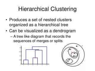
Hierarchical Clustering. Produces a set of nested clusters organized as a hierarchical tree Can be visualized as a dendrogram A tree like diagram that records the sequences of merges or splits. Strengths of Hierarchical Clustering. Do not have to assume any particular number of clusters

E N D
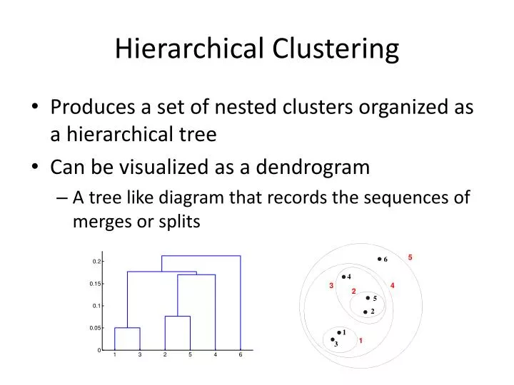
Hierarchical Clustering • Produces a set of nested clusters organized as a hierarchical tree • Can be visualized as a dendrogram • A tree like diagram that records the sequences of merges or splits
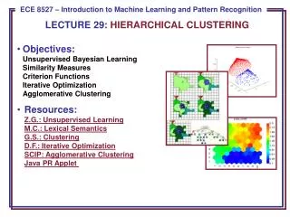
Strengths of Hierarchical Clustering • Do not have to assume any particular number of clusters • Any desired number of clusters can be obtained by ‘cutting’ the dendogram at the proper level • They may correspond to meaningful taxonomies • Example in biological sciences (e.g., animal kingdom, phylogeny reconstruction, …)
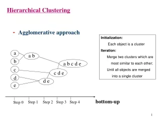
Hierarchical Clustering • Two main types of hierarchical clustering • Agglomerative: • Start with the points as individual clusters • At each step, merge the closest pair of clusters until only one cluster (or k clusters) left • Divisive: • Start with one, all-inclusive cluster • At each step, split a cluster until each cluster contains a point (or there are k clusters) • Traditional hierarchical algorithms use a similarity or distance matrix • Merge or split one cluster at a time
Agglomerative Clustering Algorithm • More popular hierarchical clustering technique • Basic algorithm is straightforward • Compute the proximity matrix • Let each data point be a cluster • Repeat • Merge the two closest clusters • Update the proximity matrix • Until only a single cluster remains • Key operation is the computation of the proximity of two clusters • Different approaches to defining the distance between clusters distinguish the different algorithms
p1 p2 p3 p4 p5 . . . p1 p2 p3 p4 p5 . . . Starting Situation • Start with clusters of individual points and a proximity matrix Proximity Matrix
C1 C2 C3 C4 C5 C1 C2 C3 C4 C5 Intermediate Situation • After some merging steps, we have some clusters C3 C4 C1 Proximity Matrix C5 C2
C1 C2 C3 C4 C5 C1 C2 C3 C4 C5 Intermediate Situation • We want to merge the two closest clusters (C2 and C5) and update the proximity matrix. C3 C4 C1 Proximity Matrix C5 C2
After Merging • The question is “How do we update the proximity matrix?” C2 U C5 C1 C3 C4 C1 ? ? ? ? ? C3 C2 U C5 C4 C3 ? ? C4 Proximity Matrix C1 C2 U C5
p1 p2 p3 p4 p5 . . . p1 p2 p3 p4 p5 . . . How to Define Inter-Cluster Similarity Similarity? • MIN • MAX • Centroid-based • Group Average • Other methods driven by an objective function • Ward’s Method uses squared error Proximity Matrix
p1 p2 p3 p4 p5 . . . p1 p2 p3 p4 p5 . . . How to Define Inter-Cluster Similarity • MIN • MAX • Centroid-based • Group Average • Other methods driven by an objective function • Ward’s Method uses squared error Proximity Matrix
p1 p2 p3 p4 p5 . . . p1 p2 p3 p4 p5 . . . How to Define Inter-Cluster Similarity • MIN • MAX • Centroid-based • Group Average • Other methods driven by an objective function • Ward’s Method uses squared error Proximity Matrix
p1 p2 p3 p4 p5 . . . p1 p2 p3 p4 p5 . . . How to Define Inter-Cluster Similarity • MIN • MAX • Centroid-based • Group Average • Other methods driven by an objective function • Ward’s Method uses squared error Proximity Matrix
p1 p2 p3 p4 p5 . . . p1 p2 p3 p4 p5 . . . How to Define Inter-Cluster Similarity Can be shown to be equivalent • MIN • MAX • Centroid-based • Group Average • Other methods driven by an objective function • Ward’s Method uses squared error Proximity Matrix
p1 p2 p3 p4 p5 . . . p1 p2 p3 p4 p5 . . . How to Define Inter-Cluster Similarity • MIN • MAX • Centroid-based • Group Average • Other methods driven by an objective function • Ward’s Method uses squared error Proximity Matrix
Usu. Called single-link to avoid confusions (min similarity or dissimilarity?) 1 2 3 4 5 Cluster Similarity: MIN or Single Link • Similarity of two clusters is based on the two most similar (closest) points in the different clusters • i.e., sim(Ci, Cj) = min(dissim(px, py)) // px Ci, py Cj = max(sim(px, py)) • Determined by one pair of points, i.e., by one link in the proximity graph.
sim(Ci, Cj) = max(sim(px, py)) Single-Link Example 0.70 0.65 0.50 0.65 0.40 1 2 3 4 5
5 1 3 5 2 1 2 3 6 4 4 Hierarchical Clustering: MIN Nested Clusters Dendrogram
Two Clusters Strength of MIN Original Points • Can handle non-elliptical shapes
Two Clusters Limitations of MIN Original Points • Sensitive to noise and outliers
1 2 3 4 5 Cluster Similarity: MAX or Complete Link • Similarity of two clusters is based on the two least similar (most distant) points in the different clusters • i.e., sim(Ci, Cj) = max(dissim(px, py)) // px Ci, py Cj = min(sim(px, py)) • Determined by all pairs of points in the two clusters
sim(Ci, Cj) = min(sim(px, py)) Complete-Link Example 0.10 0.60 0.20 0.20 0.30 1 2 3 4 5
4 1 2 5 5 2 3 6 3 1 4 Hierarchical Clustering: MAX Nested Clusters Dendrogram
Two Clusters Strength of MAX Original Points • Less susceptible to noise and outliers
Two Clusters Limitations of MAX Original Points • Tends to break large clusters • Biased towards globular clusters
Cluster Similarity: Centroid-based • Similarity of two clusters is the average of pair-wise similarity between points in the two clusters. • Can be shown to be equivalent to: 3 1 2 4 5
Centroid-based Example • sim(Ci, Cj) = avg(sim(px, py)) 3 1 2 4 5
Cluster Similarity: Group Average • GAAC (Group Average Agglomerative Clustering) • Similarity of two clusters is the average of pair-wise similarity between points in the two clusters. • Compared with the centroid-based method, this method guarantees that no inversionscan occur.
Group Average Example • sim(Ci, Cj) = avg(sim(pi, pj)) Sim(12,3)=2*(0.1+0.7+0.9)/6 = 0.5666666 3 1 2 4 5 Sim(12,45)=2*(0.9+0.65+0.2+0.6+0.5+0.8)/12 = 0.608
Hierarchical Clustering: Centroid-based and Group Average • Compromise between Single and Complete Link • Strengths • Less susceptible to noise and outliers • Limitations • Biased towards globular clusters