Download
1 / 20
340 likes | 596 Vues
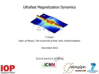
T om Ostler Dept . of Physics, The University of York, York, United Kingdom . Optical Control of Magnetization and Modeling Dynamics. Magneto-Optics/ Opto -magnetism. E. E. θ F ~M Z. Rotation ( θ f ) of polarization plane. χ : susceptibility tensor k: wave-vector n: refractive index.

E N D
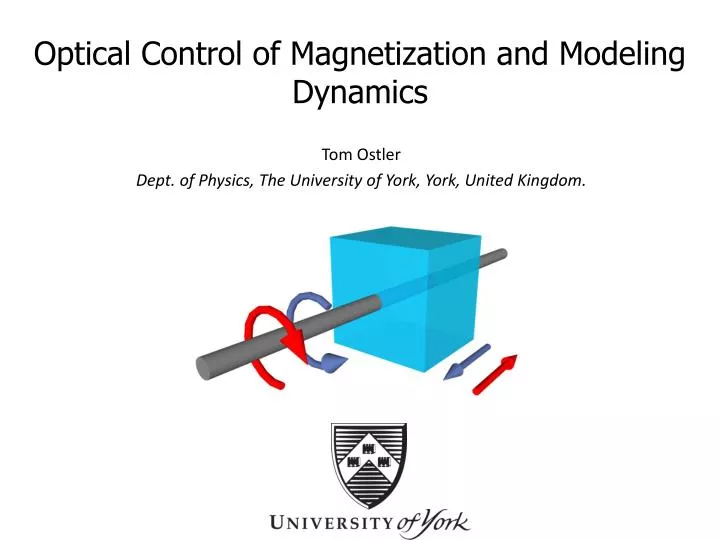
Tom Ostler Dept. of Physics, The University of York, York, United Kingdom. Optical Control of Magnetization and Modeling Dynamics
Magneto-Optics/Opto-magnetism E E θF~MZ • Rotation (θf) of polarization plane. • χ: susceptibility tensor • k: wave-vector • n: refractive index M Faraday effect • Electric field of laser radiation, E, of light induces magnetisation along k. • σ+ and σ- induce magnetisation in opposite direction σ- σ+ M(0) Inverse Faraday effect Hertel, JMMM, 303, L1-L4 (2006) *Van derZielet al., Phys Rev Lett15, 5 (1965)
Inverse Faraday Effect • Magnetization direction governed by E-field of polarized light. • Opposite helicities lead to induced magnetization in opposite direction. • Acts as “effective field” depending on helicity (±). σ+ z σ- z http://en.wikipedia.org/wiki/Circular_polarization Hertel, JMMM, 303, L1-L4 (2006)
Example: Optically Induced Precession • Light of different helicities applied to DyFeO3. • Induces spin precession with opposite phase. Kimelet al. Nature 435, 655 (2005).
Example: Optically Induced Switching • Light of different helicities applied to ferrimagneticGdFeCo. • Recall effective field opposite for σ+ and σ-. final state Initial state Stanciuet al.Phys Rev Lett, 99, 047601 (2007). *Hertel JMMM 303, L1-L4 (2006).
Linearly Polarised Light • Effective field from IFE • For σ- • For linear light (π) no effective field • What is the effect of heat and what is the role of the IFE? Hertel, JMMM, 303, L1-L4 (2006) http://en.wikipedia.org/wiki/Circular_polarization
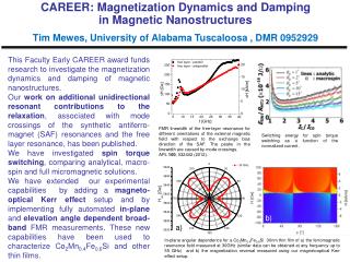
Choice of Model • Any model should be chosen carefully to include the physics important to the experiment. • Should also be appropriate to time-scale, length-scale and material. • An important aspect of femtosecond laser induced processes is including temperature into any model. TDFT/ab-initio spin dynamics 10-16 s (<fs) e-s relaxation All-optical/laser experiments Langevin Dynamics on atomistic level 10-15 s (fs) Fast-Kerr/XMCD etc 10-12 s (ps) Magnetization precession Micromagnetics/LLB Time 10-9 s (ns) 10-6 s (µs) Hysteresis Conventional magnetometers Kinetic Monte Carlo 10-3 s (ms) 10-0 s (s)+
Timescale/Lengthscale Length 10-10 m (Å) 10-9 m (nm) 10-6 m (μm) 10-3 m (mm) TDFT/ab-initio spin dynamics 10-16 s (<fs) 10-15 s (fs) Langevin Dynamics on atomiclevel 10-12 s (ps) Micromagnetics/LLB Time 10-9 s (ns) 10-6 s (µs) Kinetic Monte Carlo 10-3 s (ms) 10-0 s (s)+ http://www.psi.ch/swissfel/ultrafast-manipulation-of-the-magnetization http://www.castep.org/
Atomistic LLG & LLB for fs laser induced dynamics Langevin Dynamics on atomistic level • For each spin we solve a (coupled) LLG equation. • Different terms (zeeman, anisotropy, exchange) come in via effective field. • Includes temperature. Limited by system size. Handbook of Magnetism and Advanced Magnetic Materials (2007). • Macrospin equation Landau-Lifshitz-Bloch (macrospin) • Additional term for longitudinal relaxation unlike μmag. • Again includes temperature. Large systems. • No atomic resolution of processes. GaraninPhys Rev B, 55, 5 (1997)
Laser Heating Laser input P(t) • Two temperature model defines a temperature for conduction electrons and phonons/lattice. • Thermal term added into effective field (stochastic process). • Assume Gaussian heat pulse for laser heat. • Laser interacts directly with electronic system which has a much smaller heat capacity than phonons. • Cooling down to room temperature governed by phonon relaxation on longer time-scale. Electrons Lattice Gel e- 1500 Te e- e- 1000 e- Temp [K] Te Tl 500 energy flows Tl 0 1 2 3 *Chen et al. Journal of Heat and Mass Transfer 108, 157601 (2012). Time [ps]
IFE: Effective Field & Macrospinexample • Can add in effective field from IFE to Heff that depends on chirality. • Add Zeeman term to fields in model. • σ+ and σ- assumed to give field with opposite direction (+HOM and -HOM). • LLB (macrospin) model used to describe optical reversal in GdFeCo. • Reversal of magnetization governed by orientation of field. • Needs heat and field. Vahaplaret al. Phys Rev B 85, 104402 (2012).
LLG Example: Switching with Linearly Polarized Light Theory (atomistic LLG) • Atomistic LLG allows us to describe magnetization dynamics of individual moments. • Switching in applied field. • Linearly polarised light → heat only. Experiment • X-ray Magnetic Circular Dichroism technique. • Element specific time-resolved dynamics. • Good agreement between theory and experiment. Raduet al. Nature 472, 205-208 (2011).
Overview • Control of magnetization by circularly polarised light. • Generates an effective field dependent on chirality of light. • Have to consider transfer of heat and IFE. • When developing a model need to consider time-scale/length-scale/material. • For femtosecond laser processes macrospin (LLB) or atomistic LLG equation appropriate. • Models capable of reproducing experiment to which further analysis can be easily applied.
Controlling Transitions • (SmPr)FeO3 undergoes a gradual reorientation transtion as temperature is increased. 98 K 103 K • Above T=103 K having magnetization along ±z is energetically equivalent. • Can use polarised light to govern final state. De Jonget al. Phys Rev Lett108, 157601 (2012).
Spin moment Photons Photons Spins
Choice of Model http://www.psi.ch/swissfel/ultrafast-manipulation-of-the-magnetization http://www.castep.org/
Opto-magnetism • Light can induce a magnetization change • Change (±) depends on helicity of light • The polarised light can act as an effective field* Hertel, JMMM, 303, L1-L4 (2006) *Van derZielet al., Phys Rev Lett15, 5 (1965)
Optical Reversal: modeling Vahaplaret al. Phys Rev B 85, 104402 (2012). Laser input and effective field (IFE)
Optical Reversal: experiments and modeling • Optical stimulation of GdFeCo with σ+ and σ- measured by time-resolved Faraday effect measurements. • LLB model used to describe optical reversal in GdFeCo. • Good agreement between experiment (top) and macro-spin LLB (bottom) model. Vahaplaret al. Phys Rev B 85, 104402 (2012).