Download
1 / 34
500 likes | 836 Vues
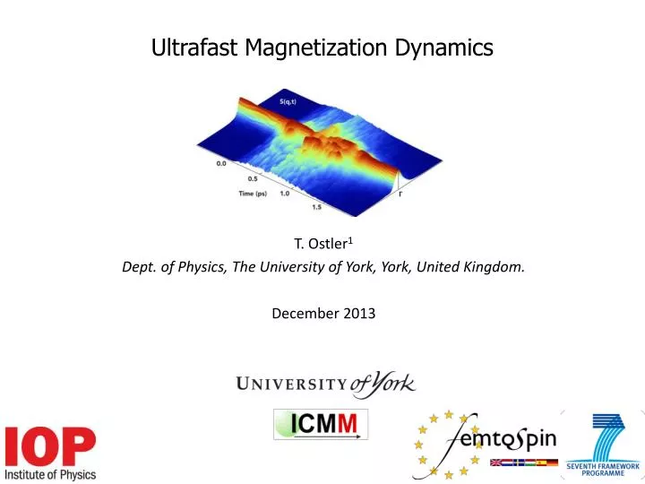
Ultrafast Magnetization Dynamics. T. Ostler 1 Dept . of Physics, The University of York, York, United Kingdom . December 2013. Increasing demand. 100TB storage. 25TB daily log. A few GB to TB’s. 2.5PB. 24PB daily. 330 EB demand in 2011. Estimated size of the internet 4ZB.

E N D
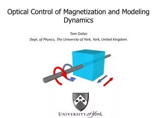
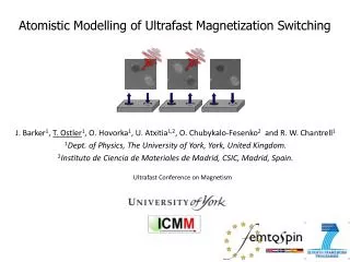
Ultrafast Magnetization Dynamics T. Ostler1 Dept. of Physics, The University of York, York, United Kingdom. December 2013
Increasing demand 100TB storage 25TB daily log A few GB to TB’s 2.5PB 24PB daily 330 EB demand in 2011 Estimated size of the internet 4ZB
Increasing demand Now at 175million Users [millions] Months • If all storage demand was met by SSD’s/flash etc, $250 billion in plant construction is required. • Faster data access/writing is desirable.
Write speed challenge • In 1953 IBM launched first commercial HHD with average data access times of just under 1 second! Me IBM 350 • A 50KB pdf would take a few days to copy. • How have data rates improved?
Speed limits in magnetism • Huge increase in speeds since the 80’s. • Rate has been slowing in last 10 years.
Write times Enterprise drive CD @ 1x How fast can we go? Faster write times Pulsed fields
Towards femtosecond processes • Magnetic field processes. • Atomistic spin dynamics model for magnetization dynamics. • LLG • How we construct such a model • Including laser heating + parameterization • Limitations of the model • Finally femtosecond lasers processes. • Conclusion: reversal in hundreds of fs using laser without applied field. • Mechanism for switching without a field.
Precession and damping • NB, if under- damped, many precesssion cycles may be necessary in order to reach equilibrium. • Current HDD has write pole around 1-2T. • Switching around 1ns. Landau-Lifshitz-Gilbert (LLG) equation Precession Damping
Ultrafast field switching in 200ps • GaAsphotoswitches excited by fs laser pulse creates initial field. • Permally thin film, in-plane. • High field and low damping causes ringing oscillations in magnetization. Figures from :Nature, 418, 509-512 (2002). • GaAsphotoswitches excited by fs laser pulse creates initial field. • Second pulses (at a very specific delay time) can stop magnetization. • Reversal complete in 200 picoseconds.
Can we go faster? • Control of magnetization dynamics in applied field limited by precession time. • There are a number of other ways to control magnetization: • Spin transfer torque • Heat assisted magnetic recording • The exchange interaction gives rise to magnetic order. • The strongest force in magnetism. Can we excite processes on this timescale? Timescale: 10’s -> 100’s fs
Femtosecond laser heating and measurement E E • Rotation (θf) of polarization plane. • χ: susceptibility tensor • k: wave-vector • n: refractive index θF~MZ M Faradayeffect Fast demagnetization of Ni • MOKE in transmission. • Using femtosecond laser pulses Beaurepaire showed fs demagnetization. • Demagnetization in around 1ps. Remagnetization in a few ps. • Can we model this? Beaurepaireet al. PRL, 76, 4250 (1996).
Time-scale/Length-scale Length 10-10 m (Å) 10-9 m (nm) 10-6 m (μm) 10-3 m (mm) TDFT/ab-initio spin dynamics 10-16 s (<fs) 10-15 s (fs) Superdiffusive spin transport 10-12 s (ps) Langevin Dynamics on atomiclevel Micromagnetics/LLB Time 10-9 s (ns) 10-6 s (µs) Kinetic Monte Carlo 10-3 s (ms) 10-0 s (s)+ http://www.psi.ch/swissfel/ultrafast-manipulation-of-the-magnetization http://www.castep.org/
The spin dynamics model • Assume fixed atomic positions • Processes such as e-e, e-p and p-p scattering are treated phenomenologically(λ). • At each timestep we calculate a field acting on each spin and solve using numerical integration. • To calculate the fields we consider a Hamiltonian (below). Extended Heisenberg Hamiltonian Exchange Anisotropy Zeeman Dipole-Dipole
How do we find J/D/μ? • Anisotropy can also be calculated from first principles. • Possible to have other anisotropy terms: • Surface • Cubic • Etc. • Jij can be found from DFT. Adiabatic approximation assuming electron motion much faster than spinwaves. • Assume frozen magnon picture • Spin spiral for particular q vector. • Integration in q-space gives exchange energy. • Can also assume nearest neighbour interaction and use experimental TC to determine Jij sc bcc fcc
Magnetization dynamics Static properties: M(T), hysteresis What can we calculate? Distribution of spinwave energies Spinwave dispersion
The spin dynamics model Heat bath • Damping is phenomenological. • Energy exchange is to/from bath and magnon-magnon interactions. Spinwaves
Modelling temperature effects Damping Precession Noise
Laser heating Chen et al. Int. Journ. Heat and Mass Transfer.49, 307-316 (2006)
How can the electron temperature be determined? Usually known from literature Fitting initial decay to an exponential Final temperature determines Figure from Atxitiaet al. Phys. Rev. B. 81, 174401 (2010).
Laser heating Experiment Theory • What governs the time-scale for demagnetization? • Can we control it? • What happens if we have multiple species?
Two sublattices Jij>0 Jij<0 Model calculations Two sublattice ferromagnet Two sublattice ferrimagnet • Strongly exchange coupled. • But decoupled dynamics. • Fine in theory, what do we see experimentally? Radu, Ostler et al. submitted.
X-ray Magnetic Circular Dichroism (XMCD) • XMCD used to measure individual magnetic elements. • Excite core electrons from spin-split valance bands. • Circularly polarized photons (+ħ,-ħ) give rise to different absorptions. Radu, Ostler et al. Nature, 472, 205-208 (2011).
Two sublattices • Experiments of dynamics (via XMCD) shows qualitatively similar results. • What determines the rate of demagnetization? Radu, Ostler et al. submitted.
Time-scales of elements in different materials • Measured demagnetization time to 50% demagnetization by tuning pump fluence. • Plot the above data against the magnetic moment. • Seems to scale with the magnetic moment. • Deviation due to exchange. Radu, Ostler et al. submitted. More details arXiv:1308.0993
Can we actually do something useful? • Controlling demagnetization is interesting but can we actually do something with it? Element-resolved dynamics. • Switching in a magnetic field • Some interesting behaviour Experiment Model results Transient ferromagnetic-like state Reversal of the sublattices Different demagnetization times Initial State Raduet al. Nature, 472, 205-208 (2011).
Switching without a field • What role is the magnetic field playing? • Model calculations show field playing almost no role! Sequence of pulses without a field Do we see the same experimentally? Ostler et al. Nat. Commun. 3, 666 (2012).
Experimental Verification: GdFeCo Microstructures Initial state - two microstructures with opposite magnetisation - Seperated by distance larger than radius (no coupling) 2mm XMCD Experimental observation of magnetisation after each pulse. Ostler et al. Nat. Commun. 3, 666 (2012).
Beyond magnetization How can we explain the observed effects in GdFeCo? Suggests something is occurring on microscopic level • No symmetry breaking external source.
Intermediate structure factor (ISF) • To obtain information on the distribution of modes in the Brillouin zone we calculate the intermediate structure factor: 3D FFT 1.0 • For each time-step we obtain S(q). • We then apply Gaussian smoothing. 0.8 0.6 Normalized Amplitude 0.4 0.2 0.0 Χ Γ Μ
Intermediate structure factor (ISF) • ISF distribution of modes even out of equilibrium. 975K Above switching threshold Below switching threshold X/2 FeCo 1090K Gd M/2 X/2 M/2 No significant change in the ISF Excited region during switching 2 bands excited • J. Barker, T. Ostler et al. Nature Scientific Reports, 3, 3262 (2013).
Dynamic structure factor (DSF) • To calculate the spinwave dispersion from the atomistic model we calculate the DSF. Relative Band Amplitude FeCo 1090K Gd X/2 M/2 • The point (in k-space) at which both bands are excited corresponds to the spinwave excitation (ISF). • J. Barker, T. Ostler et al. Nature Scientific Reports, 3, 3262 (2013).
Frequency gap • By knowing at which point in k-space the excitation occurs, we can determine a frequency (energy) gap. Overlapping bands allows for efficient transfer of energy. • This can help us understand why we do not get switching at certain concentrations of Gd. Large band gap precludes efficient energy transfer. • J. Barker, T. Ostler et al. Nature Scientific Reports, 3, 3262 (2013).
What is the significance of the excitation of both bands? • Excitation of only one band leads to demagnetization. • Excitation of both bands simultaneously leads to the transient ferromagnetic-like state. • J. Barker, T. Ostler et al. Nature Scientific Reports, 3, 3262 (2013).
Summary • Field limit of magnetization switching. • The atomistic spin dynamics model of ultrafast magnetization dynamics. • How we model femtosecond laser heating. • Demagnetization and switching experiments and theory. • How we switch without a field. Slides available at: http://tomostler.co.uk/list-of-publications/conference-presentations/