Download
1 / 107
1.09k likes | 1.28k Vues
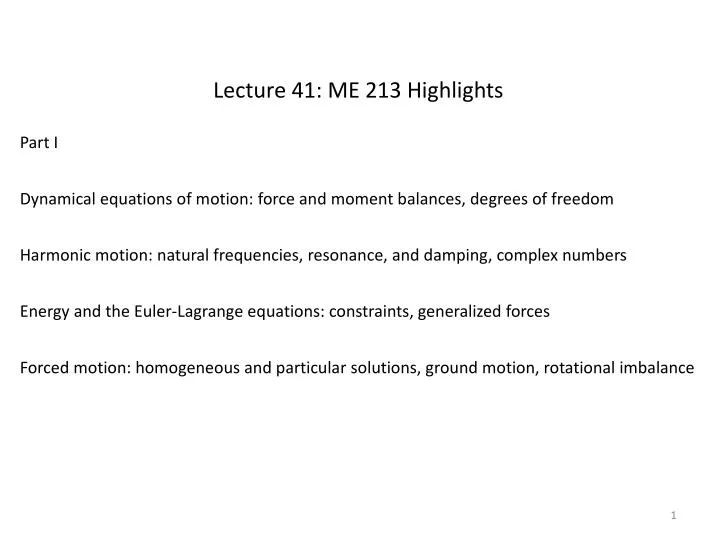
Lecture 41: ME 213 Highlights. Part I. Dynamical equations of motion: force and moment balances, degrees of freedom. Harmonic motion: natural frequencies, resonance, and damping, complex numbers. Energy and the Euler-Lagrange equations: constraints, generalized forces.

E N D
Lecture 41: ME 213 Highlights Part I Dynamical equations of motion: force and moment balances, degrees of freedom Harmonic motion: natural frequencies, resonance, and damping, complex numbers Energy and the Euler-Lagrange equations: constraints, generalized forces Forced motion: homogeneous and particular solutions, ground motion, rotational imbalance
Part II State space: conversion of mechanical and electromechanical equations Linearization: eigenvalues and eigenvectors, stability and poles Feedback control: stabilization, gains and pole placement Advanced feedback control: tracking control and observers
Dynamical equations of motion These are based on force and moment balances For simple problems free body diagrams can be used to find the equation(s) of motion The Euler-Lagrange approach is better for more complicated problems The spring force is k(y – y0) The damping force is cv, where v denotes the rate of change of y.
Dynamical equations of motion The number of degrees of freedom is the number of independent motions We had some examples back in Lecture 4, and we can look at those again now
Dynamical equations of motion We’ll limit ourselves to two dimensional motion center of mass position (y, z) orientation z q y
Dynamical equations of motion What happens when we pin a body to the world? the body has 3 DOF the pin removes two +3 -2 so we are left with = 1
Dynamical equations of motion Suppose we pin two bodies together +3 +3 -2 = 4
Dynamical equations of motion General rules for two dimensional systems Every element has three degrees of freedom to start Every pin removes 2 of them You need to think about how other constraints remove degrees of freedom For example, let’s look at the next slide
How many? Dynamical equations of motion y the floor removes two: the cart can’t move up and down the cart can’t rotate the pin removes 2 q TWO We start with six, three for each element
Dynamical equations of motion How many? one if it rolls without slipping two if it can slip three if it can leave the surface
Dynamical equations of motion How many? +3 +3 -2 -2 2
Dynamical equations of motion If I let the vertical rotate I’ll have a 3D picture that’s the base of a robot
Dynamical equations of motion The archetype of the one degree of freedom equation of motion is Undamped systems have harmonic solutions with natural frequencies define by their parameters Linearized pendulum Simple mass-spring system
Harmonic motion Harmonic motion is sinusoidal motion at a single frequency It can be written in terms of trigonometric functions or exponential functions in several equivalent ways We saw this in Lecture 2
Harmonic motion Harmonic motion is proportional to sines and cosines We can write a general harmonic function as phase amplitude frequency OR
Harmonic motion The multiple angle formulas will be very helpful You can use these to connect the two forms on the previous slide We also care about complex notation. The connections are on the next slide.
Harmonic motion Recall that so that also represents harmonic motion
imaginary axis Complex plane Harmonic motion velocity displacement blue’s the real part red’s the imaginary t real axis acceleration
Harmonic motion Phase issues sint vs. sin(t +) in the complex world
Harmonic motion Imaginary axis Complex plane resultant 1.6 exp(jwt+jf) exp(jwt) f t Real axis
Harmonic motion Real and imaginary parts
Energy and the Euler-Lagrange equations The Lagrangian, L, is the difference between the kinetic and potential energies Kinetic energy has translational and rotational components Potential energy in this course is limited to spring energy and gravitational energy Damping enters the Euler-Lagrange equations through the Rayleigh dissipation function External forcing enters through the generalized forces
Energy and the Euler-Lagrange equations ENERGY kinetic energy potential energy gravity spring
Energy and the Euler-Lagrange equations SIMPLE PENDULUM q m
Energy and the Euler-Lagrange equations FIGURE 3.1 k1 k3 k2 m1 m2 y1 y2
Energy and the Euler-Lagrange equations CONSTRAINED MOTION We need as many variables as there are degrees of freedom and NO more We can often write down the energies without reference to constraints and then we have to apply the constraints before we can go on to analysis This is often a very good thing to do!
OVERHEAD CRANE Energy and the Euler-Lagrange equations y1, f1 M but so q m (y2, z2)
Energy and the Euler-Lagrange equations DOUBLE PENDULUM q1 m1 (y1, z1) There are six variables in the figure four variables in the energy expressions and but two degrees of freedom q2 m2 (y2, z2) We probably want to use the angles as our two independent variables
Energy and the Euler-Lagrange equations z geometric constraint y differentiate q1 m1 (y1, z1) substitute and simplify q2 m2 (y2, z2)
Energy and the Euler-Lagrange equations GENERALIZED COORDINATE FORMALISM We need as many coordinates as there are degrees of freedom no more, no fewer It is traditional to name them q1, q2, etc. For the overhead crane we can put y1 = q1 and q = q2 For the double pendulum we can put q1 = q1 and q2 = q2
Energy and the Euler-Lagrange equations The energies in terms of the generalized coordinates Note the special form of T
Energy and the Euler-Lagrange equations The Lagrangian L = T - V The homogeneous Lagrange equations
Energy and the Euler-Lagrange equations The process 1. Find T and V as easily as you can 2. Apply geometric constraints to get to N coordinates 3. Assign generalized coordinates 4. Define the Lagrangian
Energy and the Euler-Lagrange equations 5. Differentiate the Lagrangian with respect to the derivative of the first generalized coordinate 6. Differentiate that result with respect to time 7. Differentiate the Lagrangian with respect to the same generalized coordinate 8. Subtract that and set the result equal to zero Repeat until you have done all the coordinates
OVERHEAD CRANE Energy and the Euler-Lagrange equations y1, f1 M Steps 1-4 lead us to q m (y2, z2)
OVERHEAD CRANE Energy and the Euler-Lagrange equations y1, f1 M but so q m (y2, z2)
Energy and the Euler-Lagrange equations The governing equations are then Put the physical variables back so it looks more familiar
Energy and the Euler-Lagrange equations Linearize (in two steps) Step one Step two: drop squares and higher products of the angles and their derivatives Final linear equations
Energy and the Euler-Lagrange equations We can find the natural frequencies of this system in the usual way There’s no damping, so we can seek harmonic solutions We can see from 8a that one of the frequencies will be zero and it represents motion of the cart with the pendulum fixed But let’s look at this more formally
Energy and the Euler-Lagrange equations Convert to an eigenvalue problem The determinant simplifies to The nonzero frequency is the square root of
Energy and the Euler-Lagrange equations We can find the zero eigenvector by inspection The other is which we can demonstrate The first row
Energy and the Euler-Lagrange equations The second row Substitute for w2 and simplify
Energy and the Euler-Lagrange equations The second motion has the cart moving in one direction and the pendulum moving in the opposite direction and the relative motion depends on the relative masses
Forced motion Put in damping and address the particular solution using complex notation m c f k
The general equation Let the forcing go like the sine Put in the complex representation of the sine We can find the solution to (3) and take the real part when we are done
Suppose that yP is proportional to the forcing function Substitute into the differential equation (3) Solve for the constant
Then we need to interpret the solution as a real quantity We need the real part of yP NOT just YP! To help us do this we need to manipulate YP
multiply top and bottom by the complex conjugate of the denominator simplify