Download
1 / 39
390 likes | 594 Vues
Synthesis of Unit Hydrographs from a Digital Elevation Model. THEODORE G. CLEVELAND, AND XIN HE University of Houston, Houston, Texas 77204 Phone: 713 743-4280, Fax: 713-743-4260 Email: cleveland@uh.edu; hexinbit@hotmail.com XING FANG Lamar University, Beaumont, Texas 77710-0024

E N D
Synthesis of Unit Hydrographs from a Digital Elevation Model THEODORE G. CLEVELAND, AND XIN HE University of Houston, Houston, Texas 77204 Phone: 713 743-4280, Fax: 713-743-4260 Email: cleveland@uh.edu; hexinbit@hotmail.com XING FANG Lamar University, Beaumont, Texas 77710-0024 Phone: 409 880-2287, Fax: 409 880-8121 Email: Xing.Fang@lamar.edu DAVID B. THOMPSON R.O. Anderson Inc., Minden, Nevada (formerly Associate Professor, Texas Tech University) Email: dthompson@roanderson.com
Acknowledgements • Texas Department of Transportation: • Transportation research projects 0-4193, 0-4194, and 0-4696. • David Stolpa, P.E., Jaime E. Villena, P.E., and George R. Herrmann, P.E., P.H. • U.S. Geologic Survey: • Dr. William Asquith, P.G., Meghan Roussel, P.E., and Amanda Garcia
Disclaimer • The contents do not reflect the official view or policies of the Texas Department of Transportation (TxDOT). • This paper does not constitute a standard, specification, or regulation.
Background and Significance • Unit hydrograph (UH) methods are used by TxDOT (and others) to obtain peak discharge and hydrograph shape for drainage design. • Drainage areas too large for rational methods. • For drainage areas small enough for lumped-parameter model. • Generally on un-gaged watersheds. • Estimating the time-response characteristics of a watershed is fundamental in rainfall-runoff modeling.
Timing Parameters • The time-response characteristics of the watershed frequently are represented by two conceptual time parameters, time of concentration (Tc) and time to peak (Tp). • Tc is typically defined as the time required for runoff to travel from the most distant point along a pathline in the watershed to the outlet. • Tp is defined as the time from the beginning of direct runoff to the peak discharge value of a unit runoff hydrograph.
Schematic • Loss model • Account for portion of rainfall that becomes available for runoff. • UH model • Temporal redistribution of the available excess precipitation at the outlet.
Loss Models • A mathematical construct that accounts for ALL rainfall losses on a watershed - the loss model does NOT redistribute the signal in time. • Proportional loss model (Univ. Houston, USGS) • Phi-index (Lamar) • Initial Abstraction - Constant Loss (USGS, TTU) • Infiltration capacity (UH, Lamar)
UH Models • A mathematical construct that accounts for temporal redistribution of the excess (after loss) rainfall signal. • Gamma unit hydrograph (USGS, Lamar) • Discrete unit hydrographs (Lamar, TTU) • Generalized gamma and geomorphic IUH (UH).
Estimating Timing Parameters • Analysis • Use actual rainfall and runoff data for a watershed. • Synthesis • Absence of data, sub-watershed, etc. • Variety of formulas for timing parameters: • Characteristic length • Characteristic slope • Flow regimes (overland, concentrated, channel) • Friction, conveyance, land type, etc. • Loss models
Estimating Timing Parameters • Representative formulas: • Overland Flow:
Estimating Timing Parameters • Representative formulas: • Channel Flow
Estimating Timing Parameters • The formulas beg the questions: • Which “lengths, slopes, friction factors” ? • What is “bankful discharge” on an ungaged watershed ? • Which “paths” to examine ?
Statistical-Mechanical Hydrograph • Leinhard (1964) postulated that the unit hydrograph is a raindrop arrival time distribution.
Statistical-Mechanical Hydrograph • Further Assumed: • The arrival time of a raindrop is proportional to the distance it must travel, l. • The number of drops arriving at the outlet in a time interval is proportional to the square of travel time (and l 2 ). • By enumerating all possible arrival time histograms, and selecting the most probable from maximum likelihood arrived at a probability distribution that represents the temporal redistribution of rainfall on the watershed.
Statistical-Mechanical Hydrograph • Resulting distribution is a generalized gamma distribution. • The distribution parameters have physical significance. • is a mean residence time of a raindrop on the watershed. • n, is an accessibility number, related to the exponent on the distance-area relationship (a shape parameter). • b, is the degree of the moment of the residence time; • b =1 is an arithmetic mean time • b =2 is a root-mean-square time
Statistical-Mechanical Hydrograph • Conventional Formulation:
Estimating Timing Parameters • The derivation based on enumeration suggests an algorithm to approximate watershed behavior. • Place many “raindrops” on the watershed. • Allow them to travel to the outlet based on some reasonable kinematics. (Explained later - significant variable is a “k” term - represents friction) • Record the cumulative arrival time. • Infer and n from the cumulative arrival time distribution. • The result is an instantaneous unit hydrograph.
Estimating Timing Parameters • Illustrate with Ash Creek Watershed • Calibration watershed – the “k” term was selected by analysis of one storm on this watershed, and applied to all developed watersheds studied. • About 7 square miles. (20,000+ different “paths”)
Estimating Timing Parameters • Place many “raindrops” on the watershed.
Estimating Timing Parameters • Allow them to travel to the outlet based on some reasonable kinematics. • Path determined by 8-cell pour point model. • Speed from quadratic-type drag, k selected to “look” like a Manning’s equation.
Estimating Timing Parameters • Allow them to travel to the outlet based on some reasonable kinematics. • Path determined by 8-cell pour point model. • Speed from local topographic slope and k • Each particle has a unique pathline. • Pathlines converge at outlet.
Estimating Timing Parameters • Record the cumulative arrival time.
Estimating Timing Parameters • Infer and n from the cumulative arrival time distribution.
Estimating Timing Parameters • The result is an instantaneous unit hydrograph (IUH). • IUH and observed storm to produce simulated runoff hydrograph. • The k is adjusted, particle tracking repeated until the observed and simulated hydrographs are the same. • This k value is then used for all watersheds. • Only change from watershed to watershed is topographic data (elevation maps)
Estimating Timing Parameters • Typical result • Ash Creek Watershed • May 1978 storm • IUH from the calibrated June 1973 storm.
Estimating Timing Parameters • Typical result • Ash Creek Watershed • May 1978 storm • IUH from the calibrated June 1973 storm.
Study Watersheds • 130+ watersheds • 2600 paired rainfall-runoff events studied. (Data base now has over 3,400 storms) • Most stations have 5 or more storms, some nearly 50 events. • Watershed boundaries, etc. determined by several methods. • Using the single value of “k” determined on the Ash Creek calibration event, applied the particle tracking approach to all developed watersheds. A second value of “k” for undeveloped watersheds is obtained from Little Elm watershed in an identical fashion.
Illustrative Results (GIUH) • Peak comparison. • Bias (low) • “k” value same all developed. • “k” value same all undeveloped.
Quantitative Results • Comparison to other methods
Conclusions • The terrain-based generates qualitatively acceptable runoff hydrographs from minimal physical detail of the watershed. • The approach simulated episodic behavior at about the same order of magnitude as observed behavior, without any attempt to account for land use.
Conclusions • For the watersheds studied, topography is a significant factor controlling runoff behavior and consequently the timing parameters common in all hydrologic models.
Publications • http://library.ctr.utexas.edu/dbtw-wpd/textbase/websearchcat.htm (Search for authors: Asquith; Roussel; Thompson; Fang; or Cleveland). • http://cleveland1.cive.uh.edu/publications (selected papers on-line). • http://infotrek.er.usgs.gov/pubs/ (Search for author Asquith; Roussel) • http://www.techmrt.ttu.edu/reports.php (Search for author Thompson) • http://ceserver.lamar.edu/People/fang/research.html