Download

1 / 53
690 likes | 1.12k Vues
Introduction to biological NMR. Dominique Marion Institut de Biologie Structurale Grenoble France. Presentation outline. Structural investigation by NMR. NMR spectral parameters. The NMR spectrometer. Two dimensional NMR. Protein HSQC. NMR resonance assignment.

E N D
Introduction to biological NMR Dominique Marion Institut de Biologie Structurale Grenoble France
Presentation outline Structural investigation by NMR NMR spectral parameters The NMR spectrometer Two dimensional NMR Protein HSQC NMR resonance assignment NMR structure calculation Protein-ligand interaction Molecular motion and relaxation
Structural investigations by NMR (1) Sample preparation (a) Optimization of the bacterial expression (b) Optimization of the protein expression (c) Labelling [15N] or [15N-13C] or [15N-13C-2H] (2) NMR experiment recording (a) Preliminary 2D experiments to optimize experimental conditions (b) 2D homonuclear experiments (< 80 aa) or 3D triple resonance experiments (>80 aa) (3) Sequential resonance assignment (a) Backbone resonances (b) Side-chain resonances
Structural investigations by NMR (4) Collection of structural restraints (a) Internuclear distances (nOe) (b) Dihedral angles (J-coupling) (c) Internuclear vector orientations (RDC) (5) Structure calculation and refinement (a) Simulated annealing (b) Structure refinement (MD simulation) (c) Structure validation (NMR statistics) (6) Complementary studies (a) Protein dynamics (Relaxation and echange) (b) Interaction with partners (ligands…)
NMR spectral parameters Shielding Chemical shift Scalar interaction J-coupling Relaxation Line-width Dipolar interaction Nuclear Overhauser effect nOe Residual dipolar coupling RDC
J-coupling NMR spectral parameters RDC Chemical shift d(ppm) 0 J+D (Hz) Nuclear Overhauser effect nOe Line-width J (Hz)
Chemical shift: ring current Upfield shifted resonance Downfield shifted resonance
J-coupling (scalar coupling) A X 1JCH > 0 J (Hz) J (Hz) Electronic cloud Electronic spin H —— C Nucleus Nuclear spin
J-couplings in 15N13C labelled proteins 1JCaCb=35Hz 2JNCa=7Hz 1JC’N=15Hz 1JCaC’=55Hz 1JNCa=11Hz 1JCaH=140Hz 2JNC’ < 1Hz 1JNH=92Hz
Nuclear Overhauser effect Relaxation in NMR: processes that allow the magnetization to return to equilibrium Origin: modulation of a spin interaction by the molecular motion S q rIS I Relaxation mechanisms in NMR: Dipole-dipole interaction Chemical shift anisotropy B0 nOe (Nuclear Overhauser effect) Transfer of nuclear magnetization from I to S via dipolar cross-relaxation
Nuclear Overhauser effect Energy diagram for a two-spin system. In small molecules with a fast tumbling rate, the transition at high frequency W2 is efficient. A population increase is observed for spin A. In large molecules with a slow tumbling Rate, the transition at low frequency W0 is efficient. A population decrease is observed for spin A. A radiofrequency field saturates the A transitions: The corresponding populations are equalized. The levels are populated according to a Boltzman distribution law.
Residual dipolar coupling Isotropic solution Weakly aligned medium S q The sign and strength of the dipolar coupling interaction between I and S depends on the relative orientation of the nuclei with respect to B0. rIS I B0 All orientation of the IS vector are equally likely. The dipolar coupling averages to zero. No structural information The proteins become weakly aligned. The dipolar coupling does not average exactly to zero. RDC structural information
Residual dipolar coupling Measured RDCs Depends upon the orientation of the internuclear vector with respect to the alignment tensor. Alignment tensor Describes the preferential orientation of the protein
J-coupling vs RDC J-couplings provide information on the relative orientation of the two internuclear vectors RDCs provide information on the absolute orientation of each internuclear vector with respect to a common molecular reference frame B0
Experimental measurement of J-coupling and nOe Continuous irradiation during spectrum recording Signal presaturation before spectrum recording
NMR spectrometer Superconducting magnet NMR console Rf generation and amplification Workstation Spectrometer control NMR probe
Superconducting magnet Insulation Dewar Liquid helium Main magnet coil Liquid nitrogen Sample NMR detection probe Magnet legs
Two-dimensional NMR [1] Preparation Evolution Mixing Detection t1 t2 The preparation and the mixing period do not change during the experiment. Jean Jeener, AMPERE Summer School in Basko Polje, Yugoslavia, September 1971
Two-dimensional NMR [2] Evolution Preparation Mixing Detection The receiver is open during the detection but not during the evolution t2 0 Dt1 t2 2Dt1 t2 3Dt1 t2
Two-dimensional NMR [3] Along t2, all the data points are recorded in real time. t1 Along t1, each data point requires a new experiment. t2
Two-dimensional NMR [4] Weak signal at the end (thermal noise) Strong signal at the beginning t1 t2
Two-dimensional NMR [5] t2 t2 t1 t1 Fourier transform along the rows Fourier transform along the columns
Two-dimensional NMR [5] t1 t2 F1 F2 t1 F2
Two-dimensional NMR [6] Chemical reaction Step 1: identification of the reactants Step 2: chemicalreaction Product Reactant Step 3: identification of the products A B More frequently: equilibrium reaction A + X B + Y
Two-dimensional NMR [7] Step 0: preparation of the reactants Step 1: identification of the reactants Reactant Product Step 2: chemicalreaction Correlation spectroscopy 3 0 1 2 Step 3: identification of the products Preparation Evolution Mixing Detection t1 t2
Two-dimensional NMR [8] Correlation spectroscopy A F1 B B B B A A B A A F2 A B Cross-peaks Preparation Evolution Mixing Detection A B Diagonal peaks t1 t2
Two-dimensional NMR [9] 1D NMR signal (in the absence of relaxation) z sin cos The NMR signal is always described as a complex number x y 2D NMR signal
Two-dimensional NMR [10] 2D NMR signal Hypercomplex data Cos (W1t1) Cos (W2t2) RR RI Cos (W1t1) Sin (W2t2) IR II Sin (W1t1) Sin (W2t2) Sin (W1t1) Cos (W2t2) Amplitude modulation
Two-dimensional NMR [11] 2D NMR signal Quadrature detection (States Method) Preparation Evolution Mixing Detection Cos (W1t1) Cos (W2t2) RR RI Cos (W1t1) Sin (W2t2) Sin (W1t1) Sin (W2t2) t1 t2 Sin (W1t1) Cos (W2t2) IR II Prep +x Prep +y
1H-15N correlation spectrum of a protein 1D cross-section along the 15N dimension 1D cross-section along the 1H dimension
1H-15N correlation spectrum of a protein Folded protein Disordered protein 179 residue fragment of hepatitis C virus non-structural protein 5A Feuerstein et al Biomol. NMR Assign. 5, 241-243 (2011). Glycine residues 175 residue imipenem-acylated L,D-transpeptidase from B. subtilis Lecoq et al Structure 20, 850-861 (2012).
NMR resonance assignment Goal: Connecting a nucleus in the protein a resonance in the spectrum
The jigsaw puzzle analogy for NMR resonance assignment When the puzzle is nearly complete, the location of the remaining pieces can be easily deduced… Two pieces have been already successfully matched Two pieces are possible candidates as neighbors on the right hand side Their shape fits roughly the profile of the already matched pair But only one piece could be anchored effortlessly This strategy is repeated for all future candidates. The useful information is not the absolute position of a piece …. But the connectivity with its neighbors.
Protein secondary structure prediction Once the resonance assignement has been obtained, the location of the secondary structure elements (a-helices and b-sheets) can be determined … without computing the complete NMR structure. TALOS + : Empirical prediction of protein [f, y] backbone torsion angles using HN, HA, CA, CB, CO, N chemical shift assignments f y a -helices Secondary structure elements in the computed structure
NMR structure calculations [1] Collecting conformational restraints Distance restraints nOe between nearby hydrogens Possible pitfalls and difficulties: – multi-spin effect or spin diffusion – conformational averaging (missing nOe) – required distance calibration Long-range and small nOe carry more structural information Separation into 3 different classes: – strong nOe (< 2.8 Å) – medium nOe ( < 3.4Å) – small nOe
NMR structure calculations [2] Collecting conformational restraints Dihedral angles Vicinal 3J coupling constant Karplus relationship Chemical shifts allow the identification of secondary structure elements Chemical shift index (CSI method) /Talos Residual dipolar coupling Finding a suitable alignment medium Protein solubility / possible alteration of the conformation
NMR structure calculations [3] Traditionalapproach for structure calculation • Collecting assigned structural information • (b) Start from a random conformation • (c) Restrained molecular dynamic with • a simplified force field. • (d) Refinement of the structure with • a complete force field and water molecules. Automatedmethods for structure calculation Automated NOESY assignment during structure calculation
NMR structure calculations [4] Resonanceassignment NOESY peakpickinglist Tentative assignment for nOes Automated methods for structure calculation Generation of a first bundle of structures Improved/extended list of nOeassignment Generation of a new set of structures
NMR structure calculations [5] Ribbonrepresentation Disordered loop Disordered N- and C-termini b-sheets a-helices Bacillus subtilis l,D-Transpeptidase 169 amino-acids
NMR and Refinement Statistics for NMR Structures Bacillus subtilis l,D-Transpeptidase 169 amino-acids Bacillus subtilis l,D-Transpeptidase 169 amino-acids Lecoq L et al. 2012. Dynamics Induced by b-Lactam Antibiotics in the Active Site of Bacillus subtilis l,D-Transpeptidase. Structure/Folding and Design 20: 850–61.
NMR and Refinement Statistics for NMR Structures Is the covalent geometry of the polypeptidic chain not distorted? What is the scattering within the set of structures that have been calculated? Is the calculated structure in agreement with the experimental data? Lecoq L et al. 2012. Dynamics Induced by b-Lactam Antibiotics in the Active Site of Bacillus subtilis l,D-Transpeptidase. Structure/Folding and Design 20: 850–61.
Protein-ligand interaction Slow exchange Fast exchange Addition of the ligand to the protein sample Observation of the protein spectrum 1D NMR or fast 2D NMR Tightbinding Weakbinding PL PL PL PL PL P + L PL P + L P P P P
Protein-ligand interaction The ligand is added to the protein: Some chemical shift variations are observed on the protein.They are located primarily at the binding interface Nuclear Overhauser effect can be observed between nuclei in the protein and in the ligand. Discrimination of intra- and intermolecular nOe is possible by means of isotopic labelling. Residual dipolar couplings can be measured for The two partners and the complex. If differences are observed, they can be explained by changes in the preferential orientation of the 2 molecules A paramagnetic tag is attached to the ligand Line-broadenings are observed on the protein at the binding interface.
Protein dynamics by NMR Protein function important role of the flexibility Protein dynamics = time dependent-fluctuations over a wide range of time scale. Ligand binding Thermostability Catalytic enzymes Folding pathways Excited states Misfolding Molten globule Conformational entropy Aggregation
NMR observables and protein motions Ligand binding Side chain rotation Protein global tumbling Enzymatic reactions Protein folding 10-12 10-9 10-6 10-3 1 103 Time (sec) EXSY RDC RT NMR T1, T2, nOe CMPG Nuclear spin relaxation Relaxation dispersion Real-time NMR
What is NMR relaxation? Longitudinal relaxation time Boltzmann equilibrium 1 – 2 exp(-t/T1) Inverted population Magnetization recovery
Molecular motion and relaxation Molecular motions in the liquid-state: Molecular motions modulate the spin interactions Internal fluctuations (side-chains, domains) Global molecular tumbling The fluctuations of the spin interaction create a local fluctuatingmagneticfield. S q rIS Here the dipolar interaction between spin I and S I B0 This fluctuatingmagneticfields push the magnetizationtowarditsequilibrium. Mz=Mz0 and Mx=My=0