Download
1 / 40
400 likes | 521 Vues
Confidence and Prediction Intervals for Small Sample Asbestos Fiber Counts based on Lognormal and Gamma Distributions. Yoonsang Kim Dulal K. Bhaumik Robert D. Gibbons. Asbestos Data.

E N D
Confidence and Prediction Intervals for Small Sample Asbestos Fiber Counts based on Lognormal and Gamma Distributions Yoonsang Kim Dulal K. Bhaumik Robert D. Gibbons
Asbestos Data • For testing and laboratory assessment, the New York State Department of Health uses various types of airborne asbestos data measured by transmission electron microscopy (TEM). • Collected as a part of the New York State Environmental Laboratory Approval Program. • All fiber counts are expressed in structures/mm2. • Amosite type used in this study. • Asbestos samples were taken from 14 different locations, which are denoted by samples, known to be contaminated • Sent to 35 laboratories to measure the fiber counts. Each asbestos sample was measured by 25 to 29 laboratories. 2
Confidence Interval • Confidence intervals for the mean asbestos fiber count are used for • if the confidence interval includes zero we do not have evidence of asbestos contamination. • if this is a health based standard or a cleanup standard, the confidence interval can be used to determine if the data are either consistent with the standard, exceed the standard, or are below the standard, and the corresponding environmental impact decision can be made. 3
Prediction Interval • Prediction intervals are useful for • testing individual new samples when a larger set of background samples are available. • Interest is in determining the probability that the new count was drawn from the distribution of the background data. • In areas where low level asbestos counts are routinely observed, prediction limits are useful for identifying new areas of possible environmental concern. 4
Introduction • For monitoring purposes, the most common measure of the asbestos concentration is the average number of counts and its upper confidence limit (UCL). • Determining the fiber count distribution is a fundamental first step in deriving a test and constructing UCL of the mean. • Asbestos fiber count (and size) data are usually right skewed. Often use the lognormal distribution to analyze. • H-statistic (Land 1973) is used to compute the UCL of the lognormal mean (EPA guidance 2002). • Finkelstein (2008) used the t-test on log-transformed asbestos fiber counts. 5
Introduction • What is the problem? • H-statistic is upward biased and difficult to implement in practice (US EPA Singh et al. 1997, Krishnamoorthy et al. 2003) • The normal distribution based approach on log-transformed data requires large sample size. (e.g. t-test) • Such data sets are typically not large enough to provide adequate power for hypothesis testing and interval estimation. 6
Introduction • The gamma distribution is widely used to analyze right-skewed data in various environmental monitoring applications. • Prediction and tolerance intervals to analyze alkalinity concentration of groundwater (Krishnamoorthy et al. 2008, Aryal et al. 2008) • US EPA proposed the use of a gamma distribution (2002) because the mean concentration may be overestimated based on the lognormal distribution (leading to an upward biased UCL). • The gamma distribution has not been used properly to characterize asbestos concentration. 7
Introduction • We propose methods for both lognormal and gamma distributions to analyze asbestos fiber counts. • Lognormal based method: the generalized confidence interval (GCI) method (Krishnamoorthy and Mathew 2003). • Gamma based method: Bhaumik et al. (2009), Krishnamoorthy et al. (2008), Aryal et al. (2008) are considered. • Compute confidence intervals and prediction intervals for data collected from the New York State Dept of Health. • Bayesian approach is also explored. 8
Lognormal distribution • Suppose X has a lognormal distribution log(X)~N(µ,σ2) • Mean of X • It is common to construct CI for E(X) based on Wald type statistic, provided the sample size is large. • Cannot obtain the correct coverage probability without large sample size. • In order to provide results for small samples, we explore the idea of generalized confidence intervals. 9
Lognormal distribution • Check if asbestos data fit to lognormal distributions. • Anderson-Darling goodness-of-fit tests for log-transformed data: normal distributions fit moderately well to 9 samples (p-values>0.09) out of a total 14 asbestos samples. • Normal quantile-quatile plot (next slide). 10
Normal Quantile-Quatile Plot for log-transformed asbestos fiber counts data Lognormal distribution doesn’t fit to samples 187Q, 7420, 5209 11
Generalized Confidence Interval • Generalized confidence interval for the mean asbestos fiber count is • Useful to construct an interval for a function of parameters of lognormal distribution, i.e., • Applicable to small sample sizes. • Easy to compute. 12
Generalized Confidence Interval • The coverage probabilities of GCI are very close to the nominal levels. • Comparison to Augus’s parametric bootstrap (1994) and Land’s (1973) methods. • Confidence limits of GCI were very close to Land’s limit. • Parametric bootstrap results were unsatisfactory for small sample size and large variance of log(X). 13
Generalized Confidence Interval • Algorithm to construct GCI for the lognormal mean. • Compute mean and variance of Y=log(X); denote them by . • Generate standard normal random variate Z and Chi-square random variate U2 with df=n-1. • Compute the generalized pivot statistic for µ+σ2/2. • Repeat steps 2 & 3 m times to obtain T1, …, Tm. • Compute 100(α/2) and 100(1–α/2) percentiles of T; denote them by Tα/2 and T1–α/2.→ CI for µ+σ2/2. • (exp(Tα/2 ), exp(T1–α/2)) is 100(1–α)% confidence interval for E(X). 14
Coverage probability for GCI • Assume the true value of . • Generate lognormal distribution with parameters . • Compute confidence interval for η following the algorithm for GCI (steps 1 to 5). • Assign 1 if the interval contains the true value of η, otherwise 0. • Repeat (ii – iv) many times (e.g., 5000 times). • Proportion of 1s is the simulated coverage probability. 16
Gamma distribution • Suppose X has a gamma distribution. Probability density function of gamma distribution is • Mean of X is • Check if asbestos data fit to lognormal distributions. • Based on Anderson-Darling goodness-of-fit tests, the gamma distribution fit 13 out 14 asbestos samples (p-values>0.15). • Gamma quantile-quantile plots (next slide). 17
Gamma Quantile-Quatile Plot for each of asbestos samples Gamma distribution does not fit to the sample 5209. 18
Gamma distribution • The confidence Interval by Bhaumik et al. (2009). • Advantages: • Type 1 error rate is better than tests previously developed for a gamma mean. • Does not depend on any unknown parameters under the null hypothesis. • Disadvantage: Slightly conservative when the true shape parameter κ is smaller than 0.5. However, for our asbestos data, the estimated shape parameter was larger than 2. 19
Coverage probability • The confidence interval was obtained by inverting the test statistic T2 for H0: E(X)=µ0 . • T2 has an approximate F distribution with df 1 and (n-1) • Coverage probability can be computed based on T2. • Generate gamma random variables with parameters . • Compute T2. If T2 falls in Fα/2 and F1–α/2 , assign 1, otherwise 0. • Repeat steps 1 and 2 many times. • Proportion of 1s is the simulated coverage proability. 21
Gamma distribution • Prediction Intervals for a single new asbestos fiber. • Krishnamoorthy, Mathew, and Mukherjee (2008) • Aryal, Bhaumik, Mathew, and Gibbons (2008) 22
Gamma distribution • Krishnamoorthy et al. (2008) • Wilson-Hilferty normal approximation used; the cubed root of a gamma random variable has an approximate normal distribution. • Suppose X is an asbestos fiber measurement and Z=X1/3. The 100(1–α)% prediction interval for X is • Advantages: • Easy to compute. • No need to estimate parameters κ and θ. • Drawback: • The lower limit can be negative (commonly set to 0). 23
Gamma distribution • Aryal et al. (2008) • A log-transformed gamma random variable has approximately a normal distribution when the shape parameter κ is large (κ>7). • The approximation normal distribution has a mean and variance, where ψ( ) is a digamma function and ψ’( )is a trigamma function. • The 100(1–α)% prediction interval for X is are maximum likelihood estimators. 24
Gamma distribution • Aryal et al. (2008) (cont.) • Advantage: • The lower limit is never negative. • Can be used even when the shape parameter κ is smaller than 7. We obtained coverage probabilities close to the nominal level when κ estimates are small too (see the table). • Drawback: • Parameters should be estimated. However, still not difficult to compute. 25
Bayesian Intervals • Specify prior knowledge about parameters or the quantity of interest as a prior density. • Miller’s (1980) conjugate prior density for the gamma parameters; • Denote X~Gamma(к,β) for 1/θ=β. The joint conjugate prior density for (к,β) with hyperparameters (p,q,r,s) is where C is a normalizing constant. • Indicates past data or hypothetical experiment with a sample size r (=s), a sum of observations q, a product of observations p. • Non-informative prior density was used. 28
Bayesian Intervals • The posterior density of (к,β) is • How to construct Bayesian confidence interval? • Simulate 10,000 draws (кℓ,βℓ) from the posterior distribution above for ℓ=1, …,10,000. • Compute кℓ/βℓfor all ℓs. These are treated as random draws from the posterior density of a gamma mean; no need to derive a posterior density of the mean. • Compute the highest posterior density (HPD) interval based on the draws к1/β1,…,к10000/β10000. This interval corresponds to the confidence interval for the mean of gamma distribution. 29
Bayesian Intervals • Highest Posterior Density (HPD) interval • Calculated in a way that values within the interval have higher probability than values outside the interval. • i.e., the HPD interval (L,U) satisfies the equation, • Used Chen and Shao’s algorithm (1999) to compute (L,U) ; built-in function in the R package boa (Smith 1997) 30
Bayesian Intervals • How to construct Bayesian prediction interval? • Simulate 10,000 draws (кℓ,βℓ) from the posterior distribution of (к,β) for ℓ=1, …,10,000. • Simulate 10,000 draws x* from then gamma density with drawn values in step 1 as parameters (i.e., from the posterior predictive density). • Compute HPD interval based on drawn values of x*. This corresponds to the prediction interval. 31
Bayesian Intervals • Asbestos sample 2778: (a) Contour plot of the joint posterior distribution of the (к,β). (b) Histogram of marginal posterior distribution of к. (c) Histogram of marginal posterior distribution of β. 32
Bayesian Intervals • Asbestos sample 2778: (d) Histogram of posterior distribution of the mean к/β; 95% HPD interval is (131.5,189.5). (e) Histogram of posterior predictive distribution for a new observation; 95% interval is (31.4, 307.1). 33
Coverage probability for Bayesian Intervals • Generate gamma data with fixed parameters (к,β) Note: this is not exactly the Bayesian idea. But this was done to compare its performance to other interval’s. • Bayesian confidence interval: • Compute HPD interval for the mean. If it contains the true value of к/β, assign 1, otherwise 0. • Repeat this many times, and compute proportion of 1s. • Bayesian prediction interval. • Compute HPD interval for a single gamma variable. • Generate a single value from gamma distribution with (к,β). • If this new single value falls in the HPD interval, assign 1. • Repeat this many times, and compute proportion of 1s. 36
Conclusion • We explored • several approaches for obtaining confidence intervals for average asbestos fiber count and • prediction intervals for a single new asbestos count • based on lognormal and gamma distributions for small samples. • Overall, Bayesian approach provides shorter length than non-Bayesian approaches, except that the length of GCI for a lognormal mean is as short as its corresponding HPD interval. • The GCI and HPD interval can be used as good alternative methods to Land’s (1973) H-statistic based confidence limit. • All methods we considered have good coverage probability. • The methods we explored can be used to characterize asbestos fiber size measurements (length and diameter). 37
Appendix 1 • AHERA: Asbestos Hazard Emergency Response Act (1986); legislation requiring the cataloging of asbestos containing building materials in schools. • Structures/mm2: asbestos structures, as defined by AHERA (fiber, bundle, matrix or cluster), per square millimeter of filter; reporting units for AHERA TEM analyses. • http://www.eia-usa.org/fact-sheets/asbestos/
Appendix 2 • Type of asbestos: The term “asbestos” refers to six fibrous minerals that have been commercially exploited and occur naturally in the environment. The U.S. Bureau of Mines has names more than 100 mineral fibers as “asbestos-like” fibers, yet only six are recognized regulated by the U.S. government. The six asbestiform minerals recognized by the government include, tremolite asbestos, actinolite asbestos, anthophyllite asbestos, chrysotile asbestos, amosite asbestos, and crocidolite asbestos. • Amosite asbestos is identified by its straight, brittle fibers that are light gray to brown in color. Amosite is also referred to as brown asbestos and its name is derived from the asbestos mines located in South Africa. In years past, amosite was often used as an insulating material and at one time it was the second-most commonly used type of asbestos. Throughout recent decades, commercial production of amosite has decreased and its use as an insulating material has been banned in many countries. • http://www.asbestos.com/asbestos/types.php
Amosite asbestos is identified by its straight, brittle fibers that are light gray to brown in color. Amosite is also referred to as brown asbestos and its name is derived from the asbestos mines located in South Africa. In years past, amosite was often used as an insulating material and at one time it was the second-most commonly used type of asbestos. Throughout recent decades, commercial production of amosite has decreased and its use as an insulating material has been banned in many countries.