Download
1 / 39
390 likes | 519 Vues
Continuous Monitoring of Nearest Neighbors on Land Surface. Presented by Ivan Chiou. Authors. Computer science department university of Southern California Los Angeles. Songhua Xing a PhD candidate at Computer Science Department now at IBM T.J. Watson Research Center

E N D
Continuous Monitoring of Nearest Neighbors on Land Surface Presented by Ivan Chiou
Authors • Computer science department university of Southern California Los Angeles. • Songhua Xing a PhD candidate at Computer Science Department now at IBM T.J. Watson Research Center Country: China • Cyrus Shahabi Director of the Information Laboratory (InfoLAB) Professor of Computer Science and Electrical Engineering at USC Director of the Integrated Media Systems Center Chief Technology Officer and Founder of Geosemble Technologies Ph.D. in Computer Science • Bei Pan a PhD candidate at Computer Science Department Microsoft Research Asia, Autodesk, University of Southern California Country:China
Abstract • New type kNN queries • Surface k Nearest Neighbor(skNN) queries • Extend to constrained third dimension • Two exact methods for highly dynamic environment as arbitrary movement • SE(Surface Expansion)-Tree • Fat and short - not efficiency • an analogous counterpart of the Dijkstra Expansion Tree on land surface • ASI(Angular Surface Index)-Tree • Thin and tall – low cpu and I/O overhead
Introduction • Related research • Static and dynamic query • Problem & Preliminaries • kNN methods only on Euclidean and road networks. • skNN is for surface distance, represented as triangular meshes. • CskNN can be used on continuous queries and the complexities of land surfaces. • CskNN algorithm • monitor and coordinate among the moving objects. • One of CkNN for road map • Dijkstra Expansion tree • SE-Tree – for Static query • More effective – ASI-Tree • Details of our surface index(ASI) and its corresponding CskNN • Dynamic query • Experiments • Summary and future work • ASI- Tree outperforms SE-Tree
Related works • Static(snapshot) query • Different constrained environment • Road networks • Land surface • Dynamic query • The paper three types of updates • Object movements • Query movements • Fluctuations of edge weights
Preliminaries • Assumption and problem definition • Moving object • Point Of Interest • Static query point • Three distance metrics • Euclidean distance • Lower bound of surface distance • Network distance • Upper bound of surface distance • Surface distance
Preliminaries • Problem definition • query consists of two steps • snapshot skNN query • continuously monitoring and updating the result sets as the objects move
Preliminaries • Shortest surface path computation • Chen-Han algorithm • costs • Unfolding process - expensive
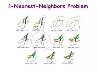
Preliminaries • Surface expansion tree • Dijkstra Expansion tree, based on the Chen-Han algorithm • Definition • Surface Expansion Tree is the final result of Chen-Han algorithm and there is only one path from the source to the vertice
Preliminaries • Surface expansion tree
Preliminaries - observation • Observation 1 makes partitioning these surface shortest paths of an SE-Tree possible. • Observation 2 Drawback • SE-Tree in general is fat and short
Naive approach • Surface Expansion Tree • Initial query processing – two areas
Object movements • Three categories • Within the result boundary • Ignore this case • Result set remains the same • Incoming movement • Outgoing movement • Two scenarios • More Outgoing movement • More Incoming movement
Naïve algorithm • Expansion phase, the complexity is • In the shrinking phase, there is no surface distance computation • Complexity is mlog(m)
Analysis – Expansion & Shrink • Similarity • All these methods built an expansion tree rooted at the query point • The result boundary and expansion boundary are the same on road networks. • Different • This naïve approach could be fast during the phase when the SE-Tree shrinks • Expansion Two problems: • Surface path computation is extremely high • Expansion areas of SE-Tree could be large. • Overcome by Surface Shortest Path Container • store partial results of pre-computation • build a novel index schema(Angular Surface Index(ASI))
SURFACE INDEX BASED ALGORITHM(1/2) • Angular Surface Index (ASI) • Thin and tall • Two data structure • Surface Shortest Path Container • Surface Equidistant Line
SURFACE INDEX BASED ALGORITHM(2/2) • Surface Shortest Path Container • To pre-compute a complete SE-Tree offline and store its shortest path. • Two Steps • locate the data object using a spatial index • retrieve the shortest path directly from disk • Drawbacks • a data object lays on the face rather than a vertex, this approach cannot find the exact shortest path and the accurate distance • storing all these shortest paths is per site • The search time is almost linear. • How to speed up • take advantage of partial results based on geometric property to speed up the online process.
Surface Shortest Path Container(1/4) • The advantage is to minimize the search area of Dijkstra algorithm. • A new concept of Cover Set and redefine the concept of Shortest Path Container for surface, and then discuss their spatial properties.
Surface Shortest Path Container(2/4) • According to Observation 1, we can always find a polyline sp from the source s to a point p on the margin of T, which is immediately left to the leftmost shortest path to CS(e) and do not cross any shortest paths, hence sp constitutes the left part of the boundary b.
Surface Shortest Path Container(3/4) • Container’s boundary consists of • the left boundary line, • the right boundary line • the end boundary line (which only exists if the left and right boundary lines do not converge)
Creating Surface Shortest Path Container • Propose an algorithm to create a surface shortest path container
Creating Surface Shortest Path Container • In Line 6, the end boundary can be NULL if left and right boundaries do not intersect the margin. • The time complexity of Algorithm 3 is O(NlogN) due to the sort operation in Line 3. However, since the pre-computation of shortest paths takes , the overall time complexity is .
Surface Equidistant Line • Designed to partition along the horizontal (latitude) direction • These lines are sorted by their increasing distance value to the source point and this order is termed as levels
Angular Surface Index(1/3) • Based on surface shortest path containers and surface equidistant lines • Each partition of is called a surface chunk. • With this ASI-Tree, each node represents a container. • Compared with SE-Tree, ASI-Tree has the following advantages
PERFORMANCE EVALUATION(1/6) • Experiment setup • Model • BH: Bearhead(BH) area in WA, USA which covers an area around 10.7km×14km and 2) • EP: Eagle Peak (EP) area in WY, USA with similar size as BH. • Create five synthetic surface models with the same size (10km×10km) • Device • PC with Intel 6420 Dual CPU • 2.13G Hz and 3.50 GB RAM • The operating system is Windows XP SP2 • The parameters • 100 CskNNqueries, each query is 50 timestamps. • The first 6 parameters are tested on both BH and EP (Surface Roughness RA is only for synthetic data sets.)
PERFORMANCE EVALUATION(2/6) • The Impact of k • ASI based algorithm outperforms the naïve algorithm both in query efficiency and I/O operations (least a factor of two for k > 4.) • Performance in I/O by an average factor of two because the search is localized to avoid unnecessary access to surface vertices.
PERFORMANCE EVALUATION(3/6) • Uniform or Gaussian distributions • the ASI based algorithm has a slightly better performance for objects with Gaussian distribution than objects with uniform distribution.
PERFORMANCE EVALUATION(4/6) • The Impact of Object Distribution and DO • Both query processing time and I/O cost decrease for both algorithms as DO increases.
PERFORMANCE EVALUATION(5/6) • The Impact of a and v • (a)(b)both query processing timeincreases slightly as well because the possibility to enlarge the search area is increased. • (c)(d)both algorithms are practically unaffected by objectspeed because the core of both algorithms only concern whetherthere are object updates rather than how far the objects move.
PERFORMANCE EVALUATION(6/6) • The Impact of DC • the performance is enhanced as more containers are created for both BH and EP. • The Impact of RA • ASI-based algorithm keeps outperforming the naïve Algorithm • rougher terrains could probably generate a largersearch area than smooth terrains.
Conclusion • Propose two algorithm • naïve algorithm • surface index (ASI) based algorithm • ASI-based algorithm outperforms the naïve algorithm under all circumstances • Simplified problem setting (pre-defined static query points)
Future work • Further studying these complex settings, where queries move arbitrarily.
BACKUP Presented by Ivan Chiou