Download
1 / 31
330 likes | 532 Vues
EET260 Frequency Modulation. Modulation. A sine wave carrier can be modulated by varying its amplitude, frequency, or phase shift. In AM, the amplitude of the carrier is modulated by a low-frequency information signal. Information signal. Amplitude modulated signal. Frequency modulation.

E N D
Modulation • A sine wave carrier can be modulated by varying its amplitude, frequency, or phase shift. • In AM, the amplitude of the carrier is modulated by a low-frequency information signal. Information signal Amplitude modulated signal
Frequency modulation • In frequency modulation (FM) the instantaneous frequency of the carrier is caused to deviate by an amount proportional to the modulating signal amplitude. instantaneous frequency changed in accordance with modulating signal frequency modulated signal
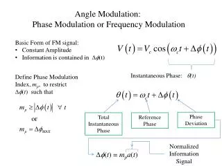
Phase modulation • In phase modulation (PM) the phase of carrier is caused to deviate by an amount proportional to the modulating signal amplitude. • Both FM and PM are collectively referred to as angle modulation. carrier phase is changed in accordance with modulating signal phase modulated signal
Frequency modulation • Consider the equation below for a frequency modulated carrier. • We will begin with a simple binary input signal. center frequency frequency deviation modulating signal defines the instantaneous frequency
Frequency modulation • We will consider a 1-V, 1-kHz square wave as an input. • Our input signal has 3 levels, and fd =4-kHz
Frequency modulation input signal (1-V, 1-kHz square wave) FM signal (fc = 10-kHz, fd = 4-kHz) f = 10-kHz f = 6-kHz f = 6-kHz f = 14-kHz f = 14-kHz f = 14-kHz
Fundamental FM concepts • The amount frequency deviation is directly proportional to the amplitude of the modulating signal. • The frequency deviation rate is determined by the frequency of the modulating signal. • The deviation rate is the number of times per second that carrier deviates above and below its center frequency. center frequency frequency deviation modulating signal
Fundamental FM concepts input signal (1-V, 1-kHz square wave) input signal (2-V, 1-kHz square wave) • Doubling the amplitude of the input doubles the frequency deviation of the carrier.
Fundamental FM concepts input signal (1-V, 1-kHz square wave) input signal (1-V, 2-kHz square wave) • Doubling the frequency of the input doubles the frequency deviation rate of the carrier.
Example Problem 1 A transmitter operates on a carrier frequency of 915-MHz. A 1-V square wave modulating signal produces 12.5-kHz deviation the carrier. The frequency of the input signal is 2-kHz. • Make a rough sketch of the FM signal. • If the modulating signal amplitude is doubled, what is the resulting carrier frequency deviation? • What is the frequency deviation rate of the carrier?
FM with sinusoidal input • Consider a sinusoidal modulating input. input signal (1-V, 500-Hz sine wave) 500-Hz modulating signal
Frequency content of an FM signal • What does an FM signal look like in the frequency domain? • We will consider the case of a sinusoidal modulating signal.
Frequency content of an AM signal Information signal vm( fim= 500-Hz ) Amplitude modulated signal vAM Modulator or mixer Frequency domain Frequency domain Frequency domain Carrier signal vc (carrier frequency fc = 5-kHz)
Frequency modulation index • The modulation index for FM is defined • Just as in AM it is used to describe the depth of modulation achieved. • From the previous example
Frequency analysis of FM • In order to determine the frequency content of we can use the Fourier series expansion given where Jn(mf)is the Bessel function of the first kind of order nand argument mf.
Frequency analysis of FM • Expanding the series, we see that a single-frequency modulating signal produces an infinite number of sets of side frequencies.
Frequency analysis of FM • Each sideband pair includes an upper and lower side frequency • The magnitudes of the side frequencies are given by coefficients Jn(m). • Although there are an infinite number of side frequencies, not all are significant.
FM spectrum for mf = 2.0 • For the case for mf = 2.0, refer to the table in Figure 5-2 to determine significant sidebands.
Bessel functions Jn(mf) if mf = 2.0, then the side frequencies we need to consider are J0, J1, J2, J3, J4
FM spectrum for mf = 2.0 • For the case for mf = 2.0, the series can be rewritten • Substituting the values for J0(2), J1(2),…, J4(2)
fc - 4fm fc - 2fm fc + 2fm fc + 4fm fc fc - 3fm fc + fm fc - fm fc + 3fm FM spectrum for mf = 2.0 • From the equation, the spectrum can be plotted. • What is the bandwidth of this signal?
FM spectrum for mf = 2.0 • The bandwidth of the previous signal is • More generally, the bandwidth is givenwhere N is the number of significant sidebands. fc - 4fm fc + 4fm
Example Problem 2 A signal vm(t) = sin (2p1000t) is frequency modulates a carrier vc(t) = sin (2p500,000t). The frequency deviation of the carrier is fd = 1000 Hz. • Determine the modulation index. • The number of sets of significant side frequencies. • Draw the frequency spectrum of the FM signal.
FM bandwidth as function of mf • FM bandwidth increases with modulation index.
FM bandwidth • Note the case mf = 0.25 • In this special case, FM produces only a single pair of significant sidebands, occupying no more bandwidth than an AM signal. • This is called narrowband FM.
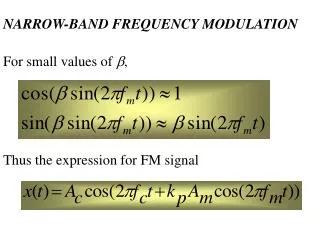
Narrowband FM • FM systems with mf <p/2 are defined as narrowband. • This is true despite the fact that only values of mf in the range of 0.2 to 0.25 have a single pair of sidebands. • The purpose of NBFM is conserve spectrum and they are widely used in mobile radios.
Carson’s Rule • An approximation for FM bandwidth is given by Carson’s rule: • The bandwidth given by Carson’s rule includes ~98% of the total power.
Example Problem 3 What is the maximum bandwidth of an FM signal with a deviation of 30 kHz and maximum modulating signal of 5 kHz as determined the following two ways: • Using the table of Bessel functions. • Using Carson’s rule.
Example Problem 3 BW = 90 kHz (Bessel functions) BW = 70 kHz (Carson’s rule)