Download
1 / 38
410 likes | 584 Vues
3D Structure calculation. In general some form of restrained Molecular Dynamics (MD) simulation is used to obtain a set of low energy structures that satisfy the NMR restraints. Procedure: Create a starting structure from sequence Optimization of the structure

E N D
In general some form of restrained Molecular Dynamics (MD) simulation is used to obtain a set of low energy structures that satisfy the NMR restraints. Procedure: Create a starting structure from sequence Optimization of the structure MD calculation with restraints from NMR Repeat this several times Selection of 'final' structures Structure Calculation
The amino acid sequence of the protein is used by the user- interface (Builder) of the modelling program to create an 'extended' starting structure. Optimization is then done by Energy Minimization (Molecular Mechanics). Starting structure and optimization
Optimized starting structure Starting structure: extended chain, often in a box of water molecules
A Molecular Dynamics Simulation is a computer calculation of the movement of the atoms in a molecule by solving Newton's equation of motion for all atoms i: (mi mass, ri position, Fi force) Molecular Dynamics Simulation
The Force Field The force Fi is calculated from tabulated potential energy terms V (the force field) and the current position ri: The empirical potential energy function V contains terms like:
Potential Energy Function Potential Energy Function for Bond Length E l l l0 Bond stretching (vibrational motion)
In addition to potentials of the force field: Non-physical restraints for distances and dihedral angles (and others) from NMR These are extra terms in the potential energy function V Restrained MD The NMR Restraints
Restraints for upper (uij) and lower (lij) bounds for the distance rij: NOE distance restraints
Molecular Dynamics Typical time-scales for molecular motions
Local or Global Energy minimum Structural landscape contains peaks and valleys. Energy Minimization protocol always moves “down hill”. Difficult to cross over local maxima to get to global minimum.
Often used with Restrained MD Potentials are 'down-scaled' in the beginning Higher degree of freedom ('sampling a bigger conformational space') In later steps the potentials are slowly brought to their final values. This is like first heating up the molecule and then cooling it down in small steps. Therefore: Simulated Annealing
Usually a large number of calculations is done in parallel resulting in a family of structures, from which an average structure can be calulated or the one with the minimum energy selected. Family of Structures Family of structures of the protein crambin
Final 3D structures of biomolecules Ribbon presentation
Choose a force-field Add constraints from NMR data Starting coordinates of all atoms (starting structure) Starting velocities of all atoms ('random seed numbers', Maxwell Boltzmann distribution) Solve Newton's classical equation of motion forvery small steps (few femto-seconds) Calculate new coordinates, forces and velocities Repeat the last two steps to find structure with lowest energy Summary: Restrained Molecular Dynamics
Advances in hardware & techniques • Higher magnetic field strength • Increased resolution & sensitivity • Maximum now 1000 MHz (1 GHz) • Cryoprobes • Cooling of probe coil with He gas (~20 K) • Reduces thermal noise generated by electric circuits • Increase of sensitivity by factor of 3-4 • Dynamic nuclear polarization (DNP) • Transferring spin polarization from electrons to nuclei • Requires saturation of electron spins by Gyrotron irradiation • So far only for solid-state NMR
Protein deuteration • Reduce 1H-1H dipolar interactions • γH/γD ~ 1/6.5 • Longer T2 → sharper lines 30 kDa 15N 15N, 90% 2H Garret DS et al. Biochemistry (1997)
TROSY 40 kDa @ 750 MHz • Transverse optimized spectroscopy • Lines from 1H-15N multiplet have differential relaxation • Interference between dipole-dipole and CSA relaxation • TROSY only selects the narrow, slowly relaxing line • TROSY effect more pronounced at high magnetic field-strength • CSA is field-dependent Pervushin K et al. PNAS (1997)
r anisotropic interactions 13C B0 CSA dipole-dipole Local fluctuating magnetic fields • Bloc(t) = Bloc[iso] + Bloc(t)[aniso] • Isotropic part is not time dependent • chemical shift • J-coupling • Only the anisotropic part is time dependent • chemical shift anisotropy (CSA) • dipolar interaction (DD)
β α non-adiabatic transitions transitions between states restore Boltzman equilibrium α β Components of the local field • Bloc(t) xy components • Transverse fluctuating fields • Non-adiabatic: exchange of energy between the spin-system and the lattice [environment] T1 relaxation
z-component: frequency ω0 varies due to local changes in B0 xy-component: transitions between states reduce phase coherence Components of the local field • Bloc(t) z component • Longitudinal fluctuating fields • Adiabatic: no exchange of energy between the spin-system and the lattice • Effective field along z-axis varies • frequency ω0 varies Bloc(t)•ez B0 adiabatic variations of ω0 T2 relaxation
Spectral density function Frequencies of the random fluctuating fields • Spectral density function J(ω) is the Fourier transform of the correlation function C(τ). It gives the probability of finding a component of the fluctuation at frequency ω. • The component of J(ω) at the Larmor frequency ω0 can induce T1 relaxation transitions. J(0) is important for T2. J(ω) τc 5 ns 10 ns 20 ns ω
Molecular tumbling and relaxation Since the integral of J(ω) over all frequencies is constant, slow tumbling (large molecule) gives more contributions at low frequencies, fast tumbling (small molecule) more at higher frequencies. J(ω) slow tumbling large protein fast tumbling small molecule Logarithmic scale
Molecular tumbling and relaxation Proteins >10kDa tc[s] correlation time fast tumbling small molecule slow tumbling large protein Inverse line width T2 ~ 1/Δn
Effects of relaxation on protein NMR spectra slower tumbling in solution fast decay of NMR signal broad lines larger number of signals more signal overlap linewidth Δν1/2 = 1/πT2 8 ns 16 kDa 25 ns 50 kDa 12 ns 24 kDa c 4 ns MW 8 kDa
Protein backbone dynamics • 15N relaxation to describe ps-ns dynamics • R1: longitudinal relaxation rate • R2: transversal relaxation rate • hetero-nuclear NOE: {1H}-15N • Measured as a 2D 1H-15N spectrum • R1,R2: Repeat experiment several times with increasing relaxation-delay • Fit the signal intensity as a function of the relaxation delay • I0. exp(-Rt) • {1H}-15N NOE: Intensity ratio between saturated and non-saturated experiment
relaxation delay 2HzNy Nx -Nz Nx 15N chemical shift evolution 15N chemical shift evolution CPMG 15N relaxation rates R2 R1 Relaxation delay
Measuring kex with CPMG • Carr-Purcell-Meiboom-Gill • Refocussing the 15N chemical shift when measuring the 15N R2 relaxation rate • Relaxation dispersion • Determine the R2,eff as a function of CPMG frequency (i.e. frequency of 180° pulses)
Relaxation dispersion Can provide information about “invisible” state • Fitting of dispersion curves at more than one magnetic field • Time-scale of the interconversion (kex=kA+kB) • Populations of the two states (pA, pB) • Chemical shift difference (Δω = ωA-ωB)
Key concepts relaxation • Wide range of time scales • Fluctuating magnetic fields • Correlation function, spectral density function • rotational correlation time (ns) • fast time scale (ps-ns): flexibility (fast backbone motions) from 15N relaxation and 1H-15N NOE • slow time scale (μs-ms): conformational exchange from relaxation dispersion CPMG