Download
1 / 37
600 likes | 1.32k Vues
Womersley Flow. Steven A. Jones BIEN 501 Wednesday, April 9, 2008. Womersley Flow. Major Learning Objectives: Apply the assumptions of Poiseuille flow to oscillating flow in a pipe. Obtain the momentum equation for this flow.

E N D
Womersley Flow Steven A. Jones BIEN 501 Wednesday, April 9, 2008 Louisiana Tech University Ruston, LA 71272
Womersley Flow Major Learning Objectives: • Apply the assumptions of Poiseuille flow to oscillating flow in a pipe. • Obtain the momentum equation for this flow. • Solve the partial differential equation through complex variables. • Relate the flow velocity profile to centerline velocity, flow rate, wall shear stress, and pressure gradient. Louisiana Tech University Ruston, LA 71272
Womersley Flow Minor Learning Objectives: • Show that the simplifications we arrived at for Poiseuille flow are consequences of fully developed flow. • Apply the momentum equation for a case that involves time and space. • Use complex analysis in the solution of a partial differential equation. • Use complex analysis to recast the solution in the form of centerline velocity instead of pressure gradient. • Apply superposition to obtain a solution for an arbitrary waveform. Louisiana Tech University Ruston, LA 71272
Womersley Flow Louisiana Tech University Ruston, LA 71272
Womersley Flow Laminar pipe flow, but with an oscillating pressure gradient, Approximation of pulsatile flow in an artery. The above “assumptions” can be obtained from the single assumption of “fully developed” flow. Louisiana Tech University Ruston, LA 71272
Fully Developed Flow In fully developed pipe flow, all velocity components are assumed to be unchanging along the axial direction, and axially symmetric i.e.: Examine continuity (for incompressible flow): 0 (no changes in z) 0 (symmetry) Louisiana Tech University Ruston, LA 71272
Fully Developed Flow From we conclude But since we have already ruled out dependence on q and z, so that f(t) must be zero. But It follows that there is no radial velocity, i.e. vr(r,t)=0. Note: It is possible to show from the q momentum equation that vq must also be zero. We will save that for a day when you really need the extra excitement. Louisiana Tech University Ruston, LA 71272
Results from Mass/Momentum Through arguments similar to the above, we find that: Now look at the z-momentum equation. Louisiana Tech University Ruston, LA 71272
Kinematic Viscosity The kinematic viscosity is defined by: Do not confuse n with the velocity v. Yes, they do look very similar, but n will not appear with a subscript. Louisiana Tech University Ruston, LA 71272
Results from Mass/Momentum The removal of the indicated terms yields: Or rearranging, and substituting for the pressure gradient: In a typical situation, we would have control over a(t). That is, we can induce a pressure gradient by altering the pressure at one end of the pipe. We will therefore take it as the input to the system (similar to what an electrical engineer might do in testing a linear system). Louisiana Tech University Ruston, LA 71272
The Pressure Gradient The form we select for the pressure gradient is: Where the subscript R represents the real part of A. Recall Euler’s rule: We also define a complex form of the axial velocity: Louisiana Tech University Ruston, LA 71272
Complex Velocity It is important to remember the following theorem: If we have a linear differential equation Where L{} is a linear differential operator, and if: Solves the equation, then the real part and the imaginary part of v(t) must satisfy the equation individually. Louisiana Tech University Ruston, LA 71272
Complex Velocity Therefore, instead of solving the equation: We can solve the equation: and take the real part of the solution afterwords to obtain the solution to: Louisiana Tech University Ruston, LA 71272
Reduction to an Ordinary Differential Equation With these concepts in mind, we substitute for the pressure gradient and for the velocity in the momentum equation. Divide by eiwt Through this process, we have removed the time dependence from the equation. This method is similar to a separation of variables method, where vz=T(t)R(r). Louisiana Tech University Ruston, LA 71272
Reduction to an Ordinary Differential Equation If we had merely assumed that vz=T(t)R(r), we would have obtained the same result. If we set The homogeneous equation is transformed into: Louisiana Tech University Ruston, LA 71272
Reduction to an Ordinary Differential Equation From /r vz r Louisiana Tech University Ruston, LA 71272
Bessel’s Equation The above equation: Should be compared to the canonical form of Bessels equation: Louisiana Tech University Ruston, LA 71272
Bessel’s Equation The solutions to Bessel’s equation are of the form: When p=0. In all cases, Yp becomes infinite at r = 0, so it is not relevant to our case. Louisiana Tech University Ruston, LA 71272
Bessel’s Equation With the homogeneous equation: Compared to the canonical form of Bessel’s equation: We can deduce that p=0 and the solution is of the form This form can be verified by substituting z=i3/2x into Bessel’s equation. Louisiana Tech University Ruston, LA 71272
Particular Solution From direct substitution, it can be verified that the particular solution to: is We can deduce that the complete solution is of the form: Louisiana Tech University Ruston, LA 71272
Ber and Bei Functions Despite the complication of the complex argument, the Bessel function above has a relatively simple formulation. The real and imaginary parts of this function are called the Ber and Bei functions, respectively. Louisiana Tech University Ruston, LA 71272
Boundary Conditions With we must satisfy the no-slip condition at r = R. Therefore, Louisiana Tech University Ruston, LA 71272
Particular Solution Equation Now back out from x to r and from y to vz. or Louisiana Tech University Ruston, LA 71272
Womersley Number The parameter Is called either the Womersley number of the alpha parameter. It is a measure of the ratio of the unsteady part of the momentum equation to the viscous part. When a is small, the unsteadiness is not important, and the solutions become parabolas (Poiseuille solutions) that vary in magnitude, but not in shape. If a is large, however, the shapes of the profiles are not parabolic. Louisiana Tech University Ruston, LA 71272
Complex Form The complex form: is less frightening than it looks. General computational software, such as MatLab has built in functions for the Bessel functions, and it can also handle the complex arithmetic. One can therefore literally program the above expression in MatLab and take the real part to obtain the physical (real) velocity. Louisiana Tech University Ruston, LA 71272
Centerline Velocity Above is the solution for velocity in terms of the pressure gradient A. What if we have a case where the pressure gradient was not measured, but the centerline velocity was. We can write an expression for velocity in terms of the centerline velocity given in the form: Louisiana Tech University Ruston, LA 71272
Centerline Velocity From the solution for velocity as a function of r and t: We would like to determine the velocity profile in terms of the centerline velocity, uz(0,t). Evaluate the above at r = 0. Louisiana Tech University Ruston, LA 71272
Centerline Velocity , so: Now note that Recall that we can talk about a complex velocity such that . Then . Louisiana Tech University Ruston, LA 71272 .
Centerline Velocity . We were not given the complex form of but we were given its magnitude (k) and phase (f), and we know that for any product of complex numbers AB, and Therefore, we can obtain the magnitude and phase of the pressure term A from as: , Louisiana Tech University Ruston, LA 71272 Since the true pressure gradient is the real part of the complex pressure gradient, we can write: .
Centerline Velocity and , Louisiana Tech University Ruston, LA 71272 Since the true pressure gradient is the real part of the complex pressure gradient, we can write: .
Centerline Velocity Since the true pressure gradient is the real part of the complex pressure gradient, we can write: . Louisiana Tech University Ruston, LA 71272
The Stress Tensor For fluids: The shear stress has 4 non-zero components. Louisiana Tech University Ruston, LA 71272
Shear Stress, Bottom Surface Along the bottom surface, we are concerned only with txy. Louisiana Tech University Ruston, LA 71272
Wall Shear Stress Similarly, we could recast the solution in the form of wall shear stress. From this simple geometry, the shear stress reduces to: To evaluate the derivative, we will need to know the derivatives of the Bessel functions. I.e. we must know that in general: so that specifically: Louisiana Tech University Ruston, LA 71272
Wall Shear Stress It is left to the student to show that: and that since: the flow rate as a function of time is: Louisiana Tech University Ruston, LA 71272
Carotid Artery Waveform A typical example of a carotid artery centerline velocity is shown here. Clearly this waveform is not a pure sine wave. It has a DC component and higher harmonics. v cm/s Time (s) Louisiana Tech University Ruston, LA 71272
Superposition If the centerline velocity is periodic. Then it can be represented as a Fourier series: Because the differential equation is linear, the solution to the above “input” is the same as the sum of solutions to each term. Thus, since we have solved the equation for a single cosine wave, we have solved them for a general case. Louisiana Tech University Ruston, LA 71272