Download
1 / 22
250 likes | 394 Vues
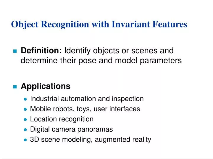
Object Recognition with Invariant Features. Definition: Identify objects or scenes and determine their pose and model parameters Applications Industrial automation and inspection Mobile robots, toys, user interfaces Location recognition Digital camera panoramas

E N D
Object Recognition with Invariant Features • Definition: Identify objects or scenes and determine their pose and model parameters • Applications • Industrial automation and inspection • Mobile robots, toys, user interfaces • Location recognition • Digital camera panoramas • 3D scene modeling, augmented reality
Cordelia Schmid & Roger Mohr (97) • Apply Harris corner detector • Use rotational invariants at corner points • However, not scale invariant. Sensitive to viewpoint and illumination change.
Invariant Local Features • Image content is transformed into local feature coordinates that are invariant to translation, rotation, scale, and other imaging parameters SIFT Features
Advantages of invariant local features • Locality: features are local, so robust to occlusion and clutter (no prior segmentation) • Distinctiveness: individual features can be matched to a large database of objects • Quantity: many features can be generated for even small objects • Efficiency: close to real-time performance • Extensibility: can easily be extended to wide range of differing feature types, with each adding robustness
Build Scale-Space Pyramid • All scales must be examined to identify scale-invariant features • An efficient function is to compute the Difference of Gaussian (DOG) pyramid (Burt & Adelson, 1983)
Key point localization • Detect maxima and minima of difference-of-Gaussian in scale space
Select canonical orientation • Create histogram of local gradient directions computed at selected scale • Assign canonical orientation at peak of smoothed histogram • Each key specifies stable 2D coordinates (x, y, scale, orientation)
Example of keypoint detection Threshold on value at DOG peak and on ratio of principle curvatures (Harris approach) • (a) 233x189 image • (b) 832 DOG extrema • (c) 729 left after peak • value threshold • (d) 536 left after testing • ratio of principle • curvatures
SIFT vector formation • Thresholded image gradients are sampled over 16x16 array of locations in scale space • Create array of orientation histograms • 8 orientations x 4x4 histogram array = 128 dimensions
Nearest-neighbor matching to feature database • Hypotheses are generated by approximate nearest neighbor matching of each feature to vectors in the database • We use best-bin-first (Beis & Lowe, 97) modification to k-d tree algorithm • Use heap data structure to identify bins in order by their distance from query point • Result: Can give speedup by factor of 1000 while finding nearest neighbor (of interest) 95% of the time
Detecting 0.1% inliers among 99.9% outliers • We need to recognize clusters of just 3 consistent features among 3000 feature match hypotheses • LMS or RANSAC would be hopeless! • Generalized Hough transform • Vote for each potential match according to model ID and pose • Insert into multiple bins to allow for error in similarity approximation • Check collisions
Probability of correct match • Compare distance of nearest neighbor to second nearest neighbor (from different object) • Threshold of 0.8 provides excellent separation
Model verification • Examine all clusters with at least 3 features • Perform least-squares affine fit to model. • Discard outliers and perform top-down check for additional features. • Evaluate probability that match is correct • Use Bayesian model, with probability that features would arise by chance if object was not present (Lowe, CVPR 01)
Solution for affine parameters • Affine transform of [x,y] to [u,v]: • Rewrite to solve for transform parameters:
3D Object Recognition • Extract outlines with background subtraction
3D Object Recognition • Only 3 keys are needed for recognition, so extra keys provide robustness • Affine model is no longer as accurate
Test of illumination invariance • Same image under differing illumination 273 keys verified in final match
Sony Aibo • (Evolution Robotics) • SIFT usage: • Recognize • charging • station • Communicate • with visual • cards