Module 8 More with Space-time Diagrams

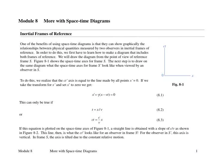
1. ct 0 x Fig. 8-1 Module 8 More with Space-time Diagrams Inertial Frames of Reference One of the benefits of using space-time diagrams is that they can show graphically the relationships between physical quantities measured by two observers in inertial frames of reference. In order to do this, we first have to learn how to make a diagram that includes both frames of reference. We will draw the diagram from the point of view of reference frame S. Figure 8-1 shows the space-time axes for frame S. The next step is to draw on the same diagram what the space-time axes for frame S’ look like when viewed by an observer in S. To do this, we realize that the ct’ axis is equal to the line made by all points x’ = 0. If we take the transform for x’ and set x’to zero we get: (8.1) This can only be true if (8.2) or (8.3) If this equation is plotted on the space-time axes of Figure 8-1, a straight line is obtained with a slope of c/v as shown in Figure 8-2. This line, then, is what the ct’looks like for an observer in frame S! For the observer in S’, this axis is vertical. In frame S, the axis is tilted due to the constant relative motion. More with Space-time Diagrams

2. ct ct’ f x’ f x Fig. 8-2 Since v < c for objects with nonzero rest masses, the slope of the ct’- axis is greater than one. Thus, the angle  between the ct and ct’ axes is less than 45. The specific value of the angle can be found by noting the slope of the ct’ line is equal to the tangent of the angle between the line and the x-axis. This angle is 90°- . Thus, (8.5) It the follows that (8.6) The next step is to draw the x’-axis as viewed in frame S. We note that the x’-axis is the line formed by all the points that have t’ = 0. Setting the transform for t’ to zero gives: (8.7) This can only be true if (8.8) or (8.9) The graph of this equation gives a line which represents the x’-axis viewed from frame S as shown in Figure 8-2. The angle between this axis and the x-axis is also equal to , the angle between the time axes. This must be true since the tangent of the angle is the slope of the x’ line. This slope is v/c. We see, then, that axes of frame S’ are tilted from the corresponding frame S axes by the angle  given by Eq. (8.6). Note that as the relative velocity between the observers increases, the angle increases and the ct’ and x’ axes rotate towards each other even more. More with Space-time Diagrams

3. ct’ 1 ct P’ 1 O x Fig. 8-3 To complete the axes in our diagram we have to know how to divide up the axes into the appropriate intervals. In other words, how long does an interval on the ct’-axis or the x’-axis appear when viewed in frame S? Let’s concentrate on the time axis first. Consider an interval of ct’ = 1. (The unit of this interval is one of length. The specific length unit doesn’t matter so let’s just drop the unit for brevity.) We know that when viewed in frame S’ this interval has a length equal to the distance from the origin O’ to the point P’ with coordinates (x’=0, ct’=1). When viewed in frame S, as depicted in Figure 8-3, this interval has a length given by the Pythagorean Theorem as (8.10) Using the transforms for x and t and with the P’ coordinates of x’=0 and ct’=1 gives (8.11) and (8.12) Substituting these values of x and t into Eq. (8.10) gives an interval length of (8.13) Note that this length is greater than one as shown in Figure 8-3. In fact, any interval on the ct’-axis appears longer by this factor in Eq. (8.13) when viewed in frame S. More with Space-time Diagrams

4. Thus, both spatial and time intervals for the frame S’ axes appear longer by this same factor of x’ P’ ct 1 O x 1 Fig. 8-4 Now let’s focus on the spatial axis. Consider an interval of x’ = 1. (Again, the unit of this interval is one of length but the specific length unit doesn’t matter so we drop the unit.) We know that when viewed in frame S’ this interval has a length equal to the distance from the origin O’ to the point P’ with coordinates (x’=1, ct’=0). When viewed in frame S, as depicted in Figure 8-4, this interval has a length given by the Pythagorean Theorem as (8.14) Using the transforms for x and t and with the P’ coordinates of x’=1 and ct’=0 gives (8.15) and (8.16) Substituting these values of x and t into Eq. (8.14) gives the same interval length we found for the time axis, namely (8.17) when viewed in frame S. More with Space-time Diagrams

5. ct ct’ and the x and x’ axes are both equal to tan-1(0.5) or 26.6°. The factor in Eq. (8.17) is equal to x’ x Fig. 8-5 26.6 5 4 4 3 3 2 2 4 1 3 1 26.6 2 1 1 2 3 4 5 We now have the necessary information to draw the axes in our space-time diagrams. As an example, consider the case where the relative velocity between the two frames is v = 0.5c. According to Eq. (8.6), the angles between the ct and ct’ axes or 1.29. Thus, the intervals on the primed axes are 1.29 longer than the intervals on the unprimed axes. This information allows us to draw the diagram shown in Figure 8.5. Note that the primed axes form angles of 26.6° with the unprimed axes and that a unit interval on a primed axis (red arrow) is 1.29 longer than a unit interval on an unprimed axis (blue arrow). Now that we know how to set up the axes, we can move on and see how the diagrams can actually be used. We’ll do that in the next section. More with Space-time Diagrams

6. ct ct ct’ ct’ P1 P2 ct1=ct2 x’ x’ x x x1 x2 Fig. 8-6 P1 P2 ct’1 ct’2 x’2 x’1 Fig. 8-7 Time and Length Revisited As examples of how we can use space-time diagrams, let’s look again at some of the principles that we developed in previous modules. For all of these examples, we’ll assume that the relative velocity between the frames is 0.5c so that the axes will look like those in Figure 8-5. We begin with the relativity of simultaneity. Suppose that two events are simultaneous in frame S. We plot the two events as P1 and P2 in Figure 8-6. Note that event 1 occurs at position x1 at time t1 and event 2 occurs at position x2 at time t2. Since the events are simultaneous, t1 = t2. We now find the times and positions of the events as seen by the observer in frame S’. To do this, we simply draw lines parallel to the primed time and position axes from the points to the axes. Where the lines intersect the axes are the corresponding times and positions of the events. This is done in Figure 8-7. We immediately see that the two events are not simultaneous in frame S’. Event 2 is observed to occur before event 1, a fact that is easily seen in the diagram. More with Space-time Diagrams

7. ct ct’ x’ x Q2 ct2 Q1 ct1 ct’1 = ct’2 x’2 x’1 x1 x2 Fig. 8-8 We can also draw the diagram for the case where two events are simultaneous in frame S’. Look at Figure 8-8. The two events, Q1 and Q2, are plotted such that they both are on a line parallel to the x’-axis. This makes both of them have the same ct’ value. To find the corresponding positions and times measured in frame S, we draw lines parallel to the unprimed axes from the points to the axes. Doing so shows that the events are not simultaneous in S and that event 1 occurs before event 2. More with Space-time Diagrams

8. ct ct Let’s next look at time dilation. Suppose an observer in frame S measures the proper time interval between two events that yields a value of ct = 1 (again with whatever length units you want). The two events must occur at the same position. When plotted on a space-time diagram, these two events might look like the points labeled P1 and P2 in Figure 8-9. Here, event 1 occurs at ct = 2 and event 2 occurs at ct = 3. Dashed lines are extended from the points to the ct’-axis parallel to the x’-axis to find the corresponding ct’ values for the two events. The size of the interval between these two times gives 1.16 on the ct’-axis. Thus, the observer in S’ measures a dilated time interval that is 1.16 times longer than the interval measured in frame S. This result agrees with the result obtained from the time dilation formula from Module 4, specifically ct’ ct’ x’ x’ where  = 1.16 for v = 0.5c. x x 6 v = 0.5c v = 0.5c 6 Q2 5 4 5 4 1.16 4 4 Q1 3 3 1.16 1.00 3 P2 3 1.00 2 2 2 P1 2 1 1 1 1 Fig. 8-9 Fig. 8-10 Let’s look at the opposite case where the observer in frame S’ measures the proper time interval. These two events would appear on the plot as the points Q1 and Q2 in Figure 8-10. The key to plotting them is that they must have the same x’ coordinate. Dashed lines are extended from the points to the ct-axis parallel to the x-axis to find the corresponding ct values. The size of the interval between these two times gives 1.16 on the ct-axis, again confirming the time dilation result! (By the way, you should confirm that both diagrams show that the observers who measure the nonproper time intervals do indeed see the two events occur at different positions. You may want to draw in the dashed lines that show this.) More with Space-time Diagrams

9. ct v = 0.5c ct’ P1 P2 Q1 x’ 0.87 4 3 2 x 1.00 1 1 2 3 4 5 Fig. 8-11 where  = 1.16 for v = 0.5c. Finally, let’s revisit length contraction and see how that looks in a space-time diagram. Suppose an observer in frame S measures the proper length of an object to be 1 (as usual, in whatever length units you want). When plotted, the two events of measuring the end positions of the object might look like the points labeled P1 and P2 in Figure 8-11. The observer in frame S’ must measure the end positions at the same time in order to get the length of the object. Let’s say that the event of measuring one end also occurs at point P2 for this observer. We know that the measuring of the other end does not occur at P1 since these two points occur correspond to different times on the ct’-axis. To find the other point, we first draw a vertical dashed line through P1 to represent the end of the object in frame S. We then draw a dashed line from P2 parallel to the x’-axis. The intersection of these two lines, Q1, is the point we are after. Notice that Q1 and P2 do occur at the same time. Now all we do is find the values of x’ for these points and measure the length of the interval between these two values. We find a length of 0.87. Thus, the observer in frame S’ measures a length that is 0.87 times the length measured by the observer in S. This agrees with the length contraction formula from Module 4, specifically Just in case you were wondering, we do get the same result if we say that the event of measuring one end of the object in S’ occurs at P1 instead of P2. You should confirm this by drawing the corresponding dashed lines on Figure 8-11. (The correct diagram appears on the next slide in Figure 8-12. Try drawing it before you click the mouse!) More with Space-time Diagrams

10. ct v = 0.5c ct’ Q2 P1 P2 x’ 0.87 4 3 2 x 1.00 1 1 2 3 4 5 Fig. 8-12 That’s it for now with the world of wonderful space-time diagrams. We next will delve into momentum and energy. But don’t forget everything you’ve learned in this module! We will use space-time diagrams in later modules to aid in our discussion of time travel. More with Space-time Diagrams